总结一些自己在实验中用到的可视化代码，以便于自己以后实验使用。

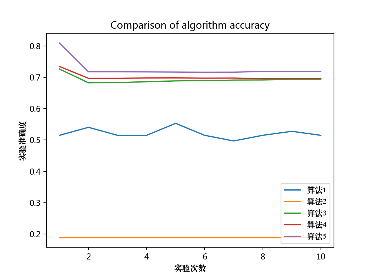
1.折线图

# %%
import matplotlib.pyplot as plt
from matplotlib.font_manager import FontProperties

#mac支持中文
font = FontProperties(fname='/Library/Fonts/Songti.ttc')

# 数据准备
x = range(1, 11)
y1 = [0.514820119, 0.540265696, 0.514820119, 0.514820119, 0.552988485, 0.514820119, 0.496779618, 0.514820119, 0.527542907, 0.514820119]
y2 = [0.188128434, 0.188128434, 0.188128434, 0.188128434, 0.188128434, 0.188128434, 0.188128434, 0.188128434, 0.188128434, 0.188128434]
y3 = [0.726365738, 0.682187617, 0.683241911, 0.685723948, 0.688467763, 0.689401198, 0.690968143, 0.691350712, 0.694016418, 0.694324856]
y4 = [0.734460903, 0.696623025, 0.696934759, 0.697733559, 0.697891845, 0.697293132, 0.697519995, 0.695791853, 0.69578938, 0.695674162]
y5 = [0.809058993, 0.717387038, 0.717405582, 0.717170923, 0.716692194, 0.715951522, 0.716337443, 0.718476258, 0.718576645, 0.718658172]

plt.plot(x, y1, label='算法1')
plt.plot(x, y2, label='算法2')
plt.plot(x, y3, label='算法3')
plt.plot(x, y4, label='算法4')
plt.plot(x, y5, label='算法5')

plt.legend(loc='lower right', prop=font)  # 让图例生效
plt.xlabel("实验次数", fontproperties=font)  # X轴标签
plt.ylabel("实验准确度", fontproperties=font)  # Y轴标签
plt.title("Comparison of algorithm accuracy")  # 标题

plt.show()

直线度分开展示

import matplotlib.pyplot as plt
from matplotlib.font_manager import FontProperties

# mac支持中文
font = FontProperties(fname='/Library/Fonts/Songti.ttc')

x = range(1, 11)
yD = [0.514820119, 0.540265696, 0.514820119, 0.514820119, 0.552988485, 0.514820119, 0.496779618, 0.514820119, 0.527542907, 0.514820119]
yE = [0.188128434, 0.188128434, 0.188128434, 0.188128434, 0.188128434, 0.188128434, 0.188128434, 0.188128434, 0.188128434, 0.188128434]
yL = [0.726365738, 0.682187617, 0.683241911, 0.685723948, 0.688467763, 0.689401198, 0.690968143, 0.691350712, 0.694016418, 0.694324856]
yR = [0.734460903, 0.696623025, 0.696934759, 0.697733559, 0.697891845, 0.697293132, 0.697519995, 0.695791853, 0.69578938, 0.695674162]
yX = [0.809058993, 0.717387038, 0.717405582, 0.717170923, 0.716692194, 0.715951522, 0.716337443, 0.718476258, 0.718576645, 0.718658172]

# 生成图片格式
fig = plt.figure()

ax1 = fig.add_subplot(121)
ax1.spines['right'].set_color('none')     # 去掉右边的边框线
ax1.spines['top'].set_color('none')       # 去掉上边的边框线
ax1.plot(x, yD, label='算法1')
ax1.plot(x, yE, label='算法2')

# 对x轴和y轴的刻度进行限制
plt.xticks(
    [0, 1, 2, 3, 4, 5, 6, 7, 8, 9, 10],
    [r'0', r'1', r'2', r'3', r'4', r'5', r'6', r'7', r'8', r'9', r'10']
)
plt.yticks(
    [0, 0.1, 0.2, 0.4, 0.5, 0.6, 0.7, 0.8],
    [r'0', r'0.1', r'0.2', r'0.3', r'0.4', r'0.5', r'0.6', r'0.7', r'0.78']
)


plt.legend(loc='up right', prop=font)  # 让图例生效
plt.xlabel(r'实验次数', fontproperties=font)  # X轴标签
plt.ylabel(r'准确度', fontproperties=font)  # Y轴标签

ax2 = fig.add_subplot(122)
ax2.spines['right'].set_color('none')     # 去掉右边的边框线
ax2.spines['top'].set_color('none')       # 去掉上边的边框线
ax2.plot(x, yL, label='算法3')
ax2.plot(x, yR, label='算法4')
ax2.plot(x, yX, label='算法5')

plt.xticks(
    [0, 1, 2, 3, 4, 5, 6, 7, 8, 9, 10],
    [r'0', r'1', r'2', r'3', r'4', r'5', r'6', r'7', r'8', r'9', r'10']
)
plt.legend(loc='up right', prop=font)  # 让图例生效
plt.xlabel(r'实验次数', fontproperties=font)  # X轴标签
# plt.xlabel("实验次数", fontproperties=font)  # X轴标签
plt.ylabel(r'准确度', fontproperties=font)  # Y轴标签
fig.suptitle(r'算法准确度对比', fontproperties=font, fontsize=15)


# 增加子图间的间隔
fig.subplots_adjust(hspace=0.4)
plt.show()

3.柱状图

import matplotlib.pyplot as plt
from matplotlib.font_manager import FontProperties

# mac支持中文
font = FontProperties(fname='/Library/Fonts/Songti.ttc')
#
Conference = {'AAAI': 18, 'ACL': 4, 'CIKM': 12, 'CogSci': 1, 'ICLR': 4, 'ICML': 6, 'IJCAI': 17, 'KDD': 31, 'NIPS': 3, 'SDM': 2, 'TKDE': 1, 'WSDM': 7, 'WWW': 6}
# 数据
x = []
y = []
for key, value in Conference.items():
    x.append(key)
    y.append(value)

# 设置图片的大小格式
plt.figure(figsize=(8, 5))

plt.bar(x, y, tick_label=x)

plt.xlabel("会议", fontproperties=font)  # X轴标签
plt.ylabel("数量", fontproperties=font)  # Y轴标签

plt.show()

4.柱状图 + 彩色

import matplotlib.pyplot as plt
import seaborn as sns
from pandas import DataFrame

plt.rc("font", family="SimHei", size="12")  # 用于解决中文显示不了的问题

# 数据
Conference = {'AAAI': 18, 'ACL': 4, 'CIKM': 12, 'CogSci': 1, 'ICLR': 4, 'ICML': 6, 'IJCAI': 17, 'KDD': 31, 'NIPS': 3, 'SDM': 2, 'TKDE': 1, 'WSDM': 7, 'WWW': 6}
x_Conference = []
y_Conference = []
for (key, value) in Conference.items():
    x_Conference.append(key)
    y_Conference.append(value)
dictionary = {'会议': x_Conference, '数量': y_Conference}
frame = DataFrame(dictionary)

# 设置图片的大小格式
plt.figure(figsize=(8, 5))

sns.barplot(x='会议', y='数量', data=frame)

plt.show()

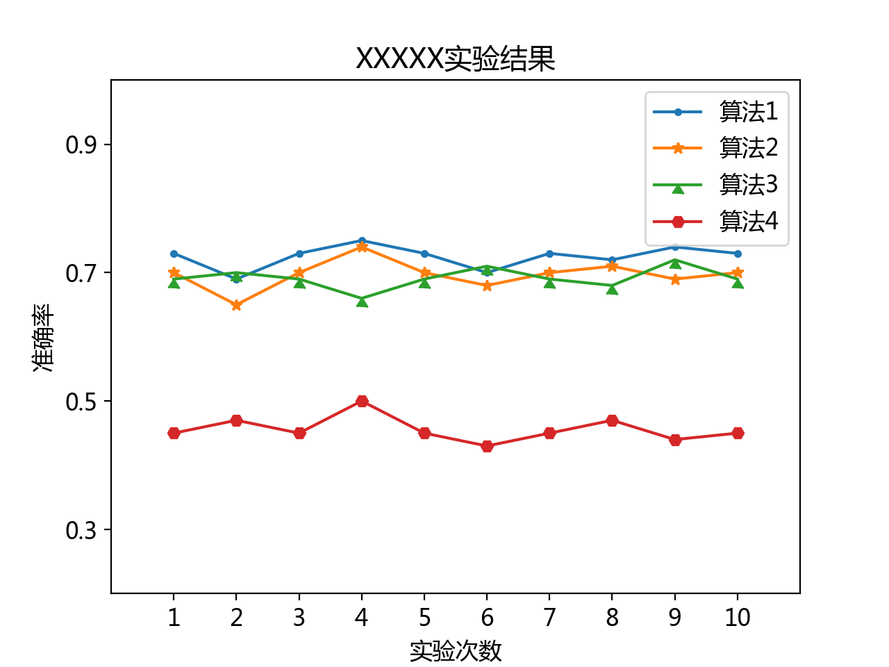
4.折线图 + 标记

import matplotlib.pyplot as plt

plt.rc("font", family="SimHei", size="12")  # 用于解决中文显示不了的问题

x = [1, 2, 3, 4, 5, 6, 7, 8, 9, 10]
y1 = [0.73, 0.69, 0.73, 0.75, 0.73, 0.70, 0.73, 0.72, 0.74, 0.73]
y2 = [0.70, 0.65, 0.70, 0.74, 0.70, 0.68, 0.70, 0.71, 0.69, 0.70]
y3 = [0.69, 0.70, 0.69, 0.66, 0.69, 0.71, 0.69, 0.68, 0.72, 0.69]
y4 = [0.45, 0.47, 0.45, 0.5, 0.45, 0.43, 0.45, 0.47, 0.44, 0.45]

plt.plot(x, y1, marker='.', label='算法1')
plt.plot(x, y2, marker='*', label='算法2')
plt.plot(x, y3, marker=6, label='算法3')
plt.plot(x, y4, marker='H', label='算法4')

plt.legend()  # 让图例生效

plt.xticks([1, 2, 3, 4, 5, 6, 7, 8, 9, 10], [r'1', r'2', r'3', r'4', r'5', r'6', r'7', r'8', r'9', r'10'])
plt.yticks([0.3,  0.5,  0.7, 0.9], [r'0.3', r'0.5', r'0.7', r'0.9'])

plt.xlim(0, 11)
plt.ylim(0.2, 1.0)

plt.xlabel("实验次数")  # X轴标签
plt.ylabel("准确率")  # Y轴标签
plt.title("XXXXX实验结果")  # 标题

plt.show()

5.散点图

import matplotlib.pyplot as plt
import numpy as np
import matplotlib

# 设置图片尺寸 8 x 4
matplotlib.rc('figure', figsize=(8, 4))
# 不显示顶部和右侧的坐标线
matplotlib.rc('axes.spines', top=False, right=False)
# 不显示网格
matplotlib.rc('axes', grid=True)

# 0.数据
x_data = np.random.rand(100) * 100
y_data = np.random.rand(100) * 100

# 1.画图
plt.scatter(x_data, y_data, s=10, color='k')
plt.title("title")
plt.xlabel("x_label")
plt.ylabel("y_label")
plt.show()

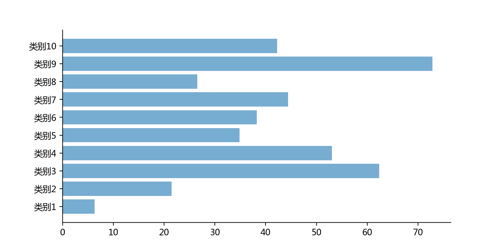
6.横向柱状图

import numpy as np
import matplotlib.pyplot as plt
import matplotlib

# 设置图片尺寸 14" x 7"
matplotlib.rc('figure', figsize=(8, 4))
# 设置字体 14
# matplotlib.rc('font', size=20)
# 不显示顶部和右侧的坐标线
matplotlib.rc('axes.spines', top=False, right=False)
# 不显示网格
matplotlib.rc('axes', grid=False)
# 设置背景颜色是白色
matplotlib.rc('axes', facecolor='white')

name = ['类别1', '类别2', '类别3', '类别4', '类别5', '类别6', '类别7', '类别8', '类别9', '类别10']

# 绘图
x = np.arange(10)
data = np.random.rand(10) * 100
plt.barh(x, data, tick_label=name, alpha=0.6)
plt.show()

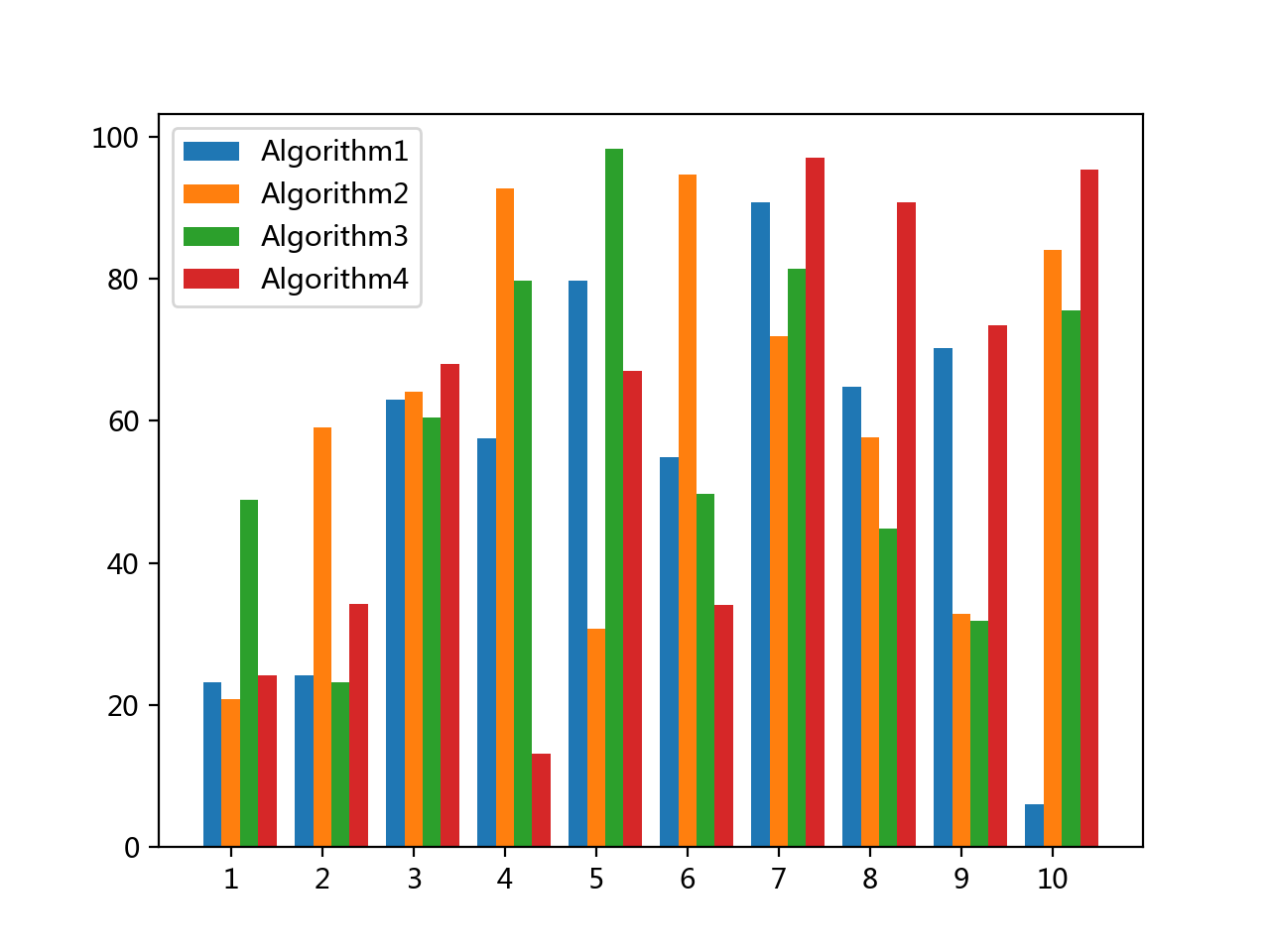
7.多柱柱状图

import matplotlib.pyplot as plt
import numpy as np

# x = [0, 1, 2, 3, 4, 5, 6, 7, 8, 9]
x_name = range(1, 11)
y1 = np.random.rand(10) * 100
y2 = np.random.rand(10) * 100
y3 = np.random.rand(10) * 100
y4 = np.random.rand(10) * 100

x = list(range(0, 10))

total_width, n = 0.8, 4
width = total_width / n


plt.bar(x, y1, width=width, label='Algorithm1')

for i in range(len(x)):
    x[i] = x[i] + width
plt.bar(x, y2, width=width, label='Algorithm2', tick_label=x_name)

for i in range(len(x)):
    x[i] = x[i] + width
plt.bar(x, y3, width=width, label='Algorithm3')

for i in range(len(x)):
    x[i] = x[i] + width
plt.bar(x, y4, width=width, label='Algorithm4')

plt.legend()
plt.show()

8.柱状图 + seaborn

import matplotlib.pyplot as plt
import seaborn as sns

data = [0.53, 0.45, 0.5, 0.40, 0.894765739, 0.89775031, 0.898468296, 0.91413729, 0.913968352, 0.913968352]

sns.countplot(data)
plt.show()

Python 数据可是化折线图、散点图、柱状图

1.折线图

直线度分开展示

3.柱状图

4.柱状图 + 彩色

4.折线图 + 标记

5.散点图

6.横向柱状图

7.多柱柱状图

8.柱状图 + seaborn

猜你喜欢

Python 数据可是化 折线图、散点图、柱状图

1.折线图

直线度分开展示

3.柱状图

4.柱状图 + 彩色

4.折线图 + 标记

5.散点图

6.横向柱状图

7.多柱柱状图

8.柱状图 + seaborn

猜你喜欢

Python 数据可是化折线图、散点图、柱状图