Table of Contents
1. 基本信息查询
导入package
import numpy as np
import matplotlib.pyplot as plt
%matplotlib inline
from sklearn import linear_model, datasets, metrics
from sklearn.neural_network import BernoulliRBM
from sklearn.pipeline import Pipeline

# 显示中文
import matplotlib as mpl
mpl.rcParams["font.sans-serif"] = ["Microsoft YaHei"]
mpl.rcParams['axes.unicode_minus'] = False
from tensorflow.examples.tutorials.mnist import input_data
data_mnist = input_data.read_data_sets(r'C:\Users\Administrator\Documents\MNIST')
Extracting C:\Users\Administrator\Documents\MNIST\train-images-idx3-ubyte.gz
Extracting C:\Users\Administrator\Documents\MNIST\train-labels-idx1-ubyte.gz
Extracting C:\Users\Administrator\Documents\MNIST\t10k-images-idx3-ubyte.gz
Extracting C:\Users\Administrator\Documents\MNIST\t10k-labels-idx1-ubyte.gz
images_all = data_mnist.train.images

images = images_all[:6000,:]
images.shape
(6000, 784)
images_X, images_y = images, data_mnist.train.labels[:6000] # 这一步为何?
np.min(images_X), np.max(images_X)
(0.0, 1.0)
plt.imshow(images_X[0].reshape(28,28), cmap=plt.cm.gray_r)
<matplotlib.image.AxesImage at 0xf8990f0>

# images_X = images_X/255.0
images_X = (images_X > 0.5).astype(float)
plt.imshow(images_X[0].reshape(28,28), cmap=plt.cm.gray_r)
<matplotlib.image.AxesImage at 0xf98c400>

2. 提取PCA 成分
假设我们从784个变量中提取100个主成分,并观察.
from sklearn.decomposition import PCA
pca = PCA(n_components=100)
pca.fit(images_X)
PCA(copy=True, iterated_power='auto', n_components=100, random_state=None,
  svd_solver='auto', tol=0.0, whiten=False)
plt.figure(figsize=(10,10))

for i, comp in enumerate(pca.components_):
    plt.subplot(10,10, i+1)
    plt.imshow(comp.reshape((28,28)), cmap=plt.cm.gray_r)
    plt.xticks(())
    plt.yticks(())
plt.suptitle('100 components by PCA')
plt.show()
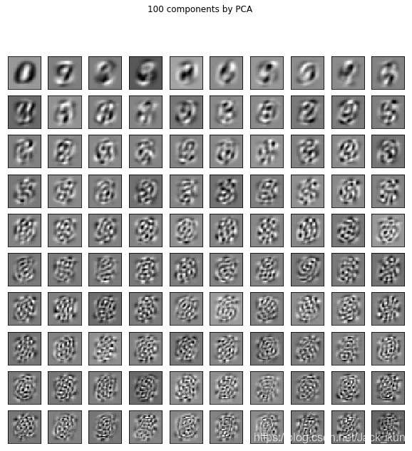
由各个特征的描述结果可以看到。前10个主成分,主要描述0,体现的是像素的一种整体形状。从后10个主成分,描述黑白像素的随机情况
pca.explained_variance_ratio_[:10].sum(),pca.explained_variance_ratio_[-10:].sum(),pca.explained_variance_ratio_[:30].sum()
(0.42493866841275713, 0.013189826871685456, 0.6406096747833725)
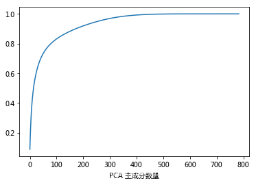
前30%的主成分解释了原有数据的64%的信息
full_pca = PCA(n_components=784)
full_pca.fit(images_X)
plt.plot(np.cumsum(full_pca.explained_variance_ratio_))
plt.xlabel('PCA 主成分数量')
<matplotlib.text.Text at 0x19c17eb8>
pca.transform(images_X[:1])
array([[ 0.52356293,  1.72349003, -2.14897954,  2.68673318,  0.47904816,
        -1.23169352,  1.04362899,  1.41068746,  1.21128259,  0.74175855,
         1.64123539, -3.34081047, -0.68832884,  0.03740046, -0.31612483,
         0.95930869,  0.75656307,  0.85933748,  1.06149407, -0.10313465,
         0.39483926,  1.68371086, -1.07682393, -0.257166  , -0.86288074,
         1.71591167, -0.62275775,  1.10727832,  0.53435806,  1.46806889,
         0.84523054,  0.71653435,  0.26125092,  0.65679105,  0.02417695,
         0.54178825,  0.09140743, -0.47275769,  0.22448948,  1.32993595,
        -1.36367223,  0.21807472,  0.93320535, -0.0499107 , -0.92103529,
        -0.43783948,  0.24625445,  0.77436417,  0.59435984, -0.33551929,
        -0.11900602, -0.94889884, -0.99956816, -0.43388146,  0.3136769 ,
        -0.50563104, -0.57570834, -0.26703065, -0.28846614, -0.59134512,
        -0.42216871, -0.70174101, -0.49465544, -0.14962569,  0.67165476,
         0.03205398,  0.11720721, -0.33503693,  0.11959339, -0.56115567,
        -0.16465967, -0.25587122,  0.48418026, -0.3838457 , -0.16103517,
         0.52447191, -0.72697503, -0.26878197,  0.36217831, -0.27052404,
         0.48639081,  0.39132248, -0.02694144, -0.33737552,  0.1130496 ,
        -0.00843058,  0.29904734,  0.92900628, -0.07937508, -0.67891584,
        -0.34406307, -0.24891354, -0.08196933,  0.17025649, -0.08947269,
         0.01181867, -0.03082805,  0.55370055,  0.22111017, -0.1240324 ]])
3. 提取RBM主成分
成分数量100,迭代次数20,随机因子设定
rbm = BernoulliRBM(random_state=0, verbose=True, n_iter=20, n_components=100)
rbm.fit(images_X)
[BernoulliRBM] Iteration 1, pseudo-likelihood = -142.78, time = 4.39s
[BernoulliRBM] Iteration 2, pseudo-likelihood = -132.65, time = 4.83s
[BernoulliRBM] Iteration 3, pseudo-likelihood = -125.75, time = 3.94s
[BernoulliRBM] Iteration 4, pseudo-likelihood = -123.83, time = 3.84s
[BernoulliRBM] Iteration 5, pseudo-likelihood = -117.85, time = 4.77s
[BernoulliRBM] Iteration 6, pseudo-likelihood = -129.62, time = 8.42s
[BernoulliRBM] Iteration 7, pseudo-likelihood = -114.95, time = 5.17s
[BernoulliRBM] Iteration 8, pseudo-likelihood = -113.14, time = 5.54s
[BernoulliRBM] Iteration 9, pseudo-likelihood = -119.25, time = 5.78s
[BernoulliRBM] Iteration 10, pseudo-likelihood = -118.98, time = 3.98s
[BernoulliRBM] Iteration 11, pseudo-likelihood = -115.08, time = 4.07s
[BernoulliRBM] Iteration 12, pseudo-likelihood = -116.79, time = 4.02s
[BernoulliRBM] Iteration 13, pseudo-likelihood = -120.36, time = 5.32s
[BernoulliRBM] Iteration 14, pseudo-likelihood = -120.43, time = 3.83s
[BernoulliRBM] Iteration 15, pseudo-likelihood = -117.06, time = 3.75s
[BernoulliRBM] Iteration 16, pseudo-likelihood = -126.19, time = 3.73s
[BernoulliRBM] Iteration 17, pseudo-likelihood = -123.19, time = 3.82s
[BernoulliRBM] Iteration 18, pseudo-likelihood = -115.31, time = 3.89s
[BernoulliRBM] Iteration 19, pseudo-likelihood = -113.10, time = 3.83s
[BernoulliRBM] Iteration 20, pseudo-likelihood = -117.98, time = 3.80s


BernoulliRBM(batch_size=10, learning_rate=0.1, n_components=100, n_iter=20,
       random_state=0, verbose=True)
plt.figure(figsize=(10,10))
for i, comp in enumerate(rbm.components_):
    plt.subplot(10, 10, i+1)
    plt.imshow(comp.reshape((28,28)), cmap=plt.cm.gray_r)
plt.xticks()
plt.yticks()
plt.suptitle('100 主成分 by RBM')
plt.show()
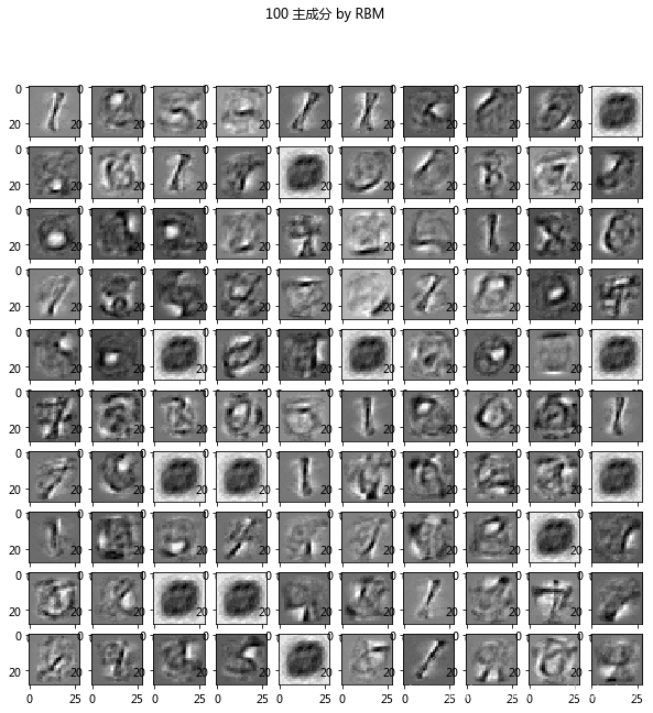
从上面观察的话,有部分的主成分是相似的,但真实值是有区别。
image_new_features = rbm.transform(images_X[:1]).reshape(100,)
image_new_features
array([  7.76673604e-15,   1.49069292e-06,   9.55226339e-11,
         9.99989771e-01,   7.57901771e-17,   1.28364972e-18,
         1.16423303e-18,   1.85040066e-19,   1.64562339e-33,
         9.99999965e-01,   1.00000000e+00,   1.30547116e-11,
         2.25132935e-18,   3.92508207e-26,   9.99999994e-01,
         1.43402544e-26,   1.46179051e-24,   2.40049579e-13,
         6.08933225e-02,   5.49458550e-22,   1.39120674e-18,
         9.99999959e-01,   1.00000000e+00,   7.54435384e-02,
         5.68688998e-13,   1.00000000e+00,   1.40116926e-09,
         1.32911930e-14,   1.66657538e-08,   1.01839668e-14,
         6.20364773e-22,   4.80370202e-21,   1.00000000e+00,
         9.99986780e-01,   9.68360209e-01,   1.00000000e+00,
         8.72995544e-13,   3.00381851e-17,   9.99813915e-01,
         2.36386359e-17,   7.22854123e-01,   4.08520026e-18,
         9.99999867e-01,   1.67875177e-17,   6.99195965e-03,
         9.99999980e-01,   9.99999354e-01,   4.09705958e-21,
         6.29987342e-12,   9.99999945e-01,   8.19464506e-12,
         5.72527937e-07,   1.04592638e-06,   2.06074887e-08,
         2.08771197e-04,   4.46575921e-17,   5.15385587e-09,
         9.07210343e-08,   1.30004168e-02,   1.15188762e-17,
         4.72222949e-15,   4.09872360e-10,   9.99999895e-01,
         9.99999995e-01,   4.59721307e-17,   9.99917857e-01,
         1.00000000e+00,   1.09751419e-03,   2.10415770e-09,
         9.99999990e-01,   1.45240705e-07,   4.22687339e-01,
         9.99998734e-01,   1.53904429e-07,   3.75029784e-25,
         1.62168712e-26,   9.99999999e-01,   6.24449101e-15,
         9.99999795e-01,   2.08631558e-19,   2.33601220e-14,
         4.63712966e-26,   9.99999875e-01,   9.99999984e-01,
         1.00000000e+00,   7.02768473e-13,   3.34203731e-16,
         9.99999632e-01,   9.99998566e-01,   5.20516733e-16,
         2.77826938e-11,   8.65331812e-07,   1.14021791e-09,
         1.12107682e-17,   9.99999829e-01,   8.97988679e-14,
         1.13375304e-13,   4.73292411e-07,   4.15078855e-02,
         9.86210789e-01])
np.dot(images_X[:1]-images_X.mean(axis=0), rbm.components_.T)
array([[ -4.35640343,   3.09815273,  -8.96732465,  16.16171671,
         -0.92552752, -11.3936493 , -17.66878685, -31.05364275,
        -55.58072995,  -3.33167638,  49.21657951, -15.98488937,
        -11.66679346, -37.654284  ,  -3.40367975, -37.89639958,
        -28.41722901, -10.87301095, -12.22387153, -17.46112116,
          1.84502414,  20.26603895,  46.54081239,   8.3612151 ,
         -2.25039004,  15.75994935,   0.92477231,  -4.2922096 ,
          3.67487237, -16.17087459, -18.88340271, -31.12333759,
         59.82613022,  31.04368552,  35.17320636,  46.02308762,
         -2.50456561, -25.90799767,  28.33256117, -18.1128016 ,
         27.21562369, -11.60404548,  -2.83829775,  -7.10104947,
          3.00935928,  -2.89662714,  12.01018771, -19.25349294,
        -21.81753662,  -3.0530714 ,   4.68355653, -14.13733712,
          2.46498274, -10.74595849,  14.52808854,  -2.79228021,
         -9.30113454,   5.32310421,  -1.07884352,  -7.18723205,
         -4.77835331,  -0.88611728,  -3.32560852,  -3.57722757,
         -7.94020713,  20.34851985,  32.38229912,   4.76989267,
         -9.13085228,  -3.3097796 ,   6.96496308,  -3.87208876,
         30.98690441,   3.43280247, -32.71121127, -39.74467406,
         38.33315289, -14.95538716,  -3.02767468, -32.54087139,
        -16.69611143, -37.44597534,  -3.24721591,  -3.1051272 ,
         53.66291505, -14.494897  ,  -6.55842747,  31.50690171,
         44.2169187 , -13.41007469, -12.01283844,   4.12374268,
         -1.05586219, -15.06200184,  -2.90743519,  -4.20470404,
          3.3775784 ,   7.99768637,   7.28527442,  32.10640592]])
注意:RBM中的transform方法并未实现center的操作,有别与PCA中的。
扫描二维码关注公众号,回复:
4834950 查看本文章

取出前20个最有代表性的特征
top_features = image_new_features.argsort()[-20:][::-1]
top_features
array([35, 10, 84, 22, 32, 66, 25, 76, 63, 14, 69, 83, 45,  9, 21, 49, 62,
       82, 42, 94], dtype=int64)
image_new_features[top_features]
array([ 1.        ,  1.        ,  1.        ,  1.        ,  1.        ,
        1.        ,  1.        ,  1.        ,  1.        ,  0.99999999,
        0.99999999,  0.99999998,  0.99999998,  0.99999996,  0.99999996,
        0.99999995,  0.99999989,  0.99999988,  0.99999987,  0.99999983])
说明这里有9个特征具有100%的解释性
plt.figure(figsize=(25,25))
for i, comp in enumerate(top_features):
    plt.subplot(5,4,i+1)
    plt.imshow(rbm.components_[comp].reshape((28,28)), cmap=plt.cm.gray_r)
    plt.title('component {}, feature value:{}'.format(comp, round(image_new_features[comp],2)), fontsize=20)
plt.xticks()
plt.yticks()
plt.suptitle('top20的主成分 by RBM')
plt.show()
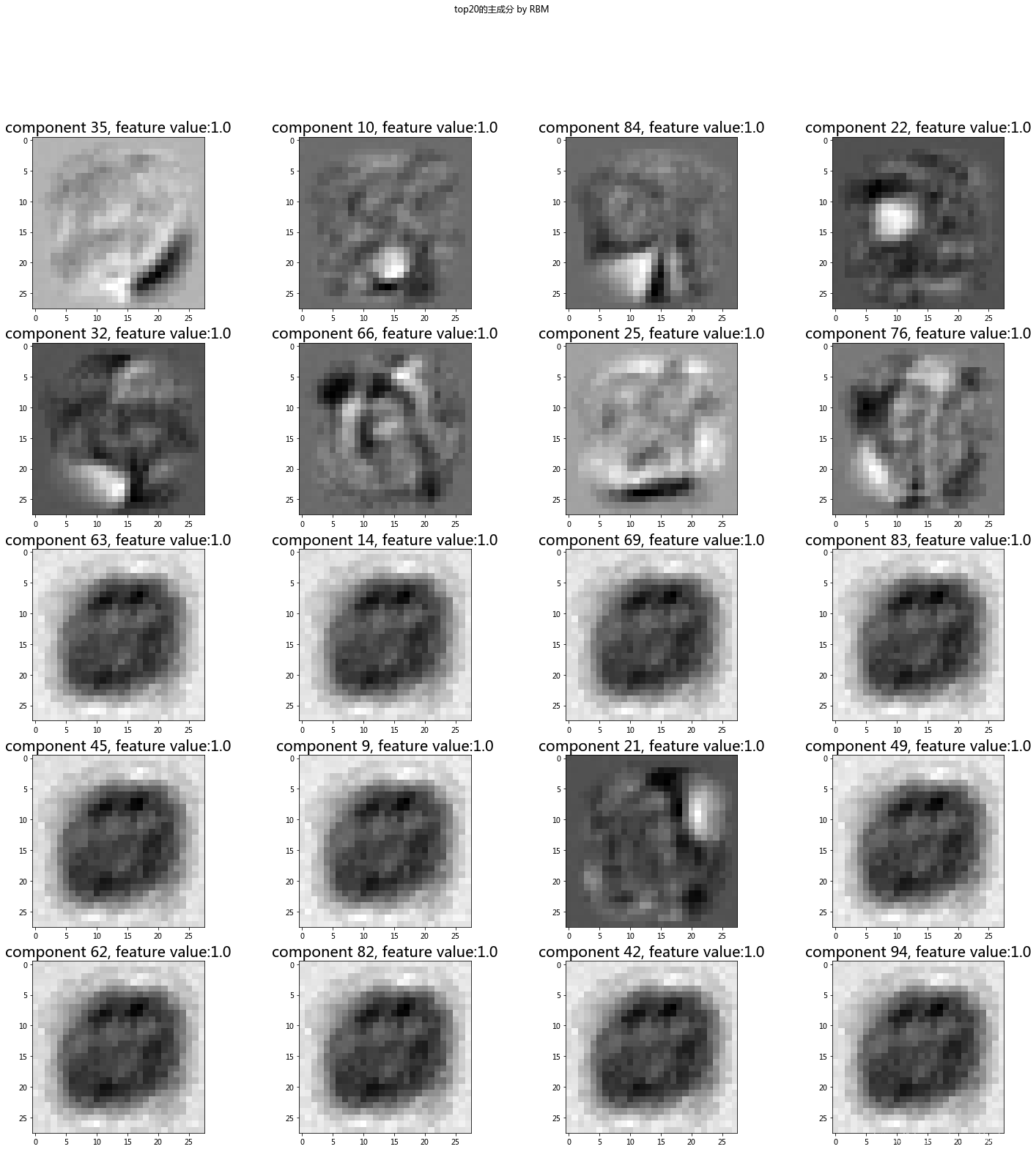
63,14,69,83都希望能直接获取3的值
25获取底部的特征
35获取右下角的特征
提取后20个特征
least_features = image_new_features.argsort()[:20][::-1]
least_features
array([59, 93, 41, 12, 20,  5,  6, 79,  7, 31, 47, 30, 19, 16, 74, 81, 13,
       75, 15,  8], dtype=int64)
image_new_features[least_features]
array([  1.15188762e-17,   1.12107682e-17,   4.08520026e-18,
         2.25132935e-18,   1.39120674e-18,   1.28364972e-18,
         1.16423303e-18,   2.08631558e-19,   1.85040066e-19,
         4.80370202e-21,   4.09705958e-21,   6.20364773e-22,
         5.49458550e-22,   1.46179051e-24,   3.75029784e-25,
         4.63712966e-26,   3.92508207e-26,   1.62168712e-26,
         1.43402544e-26,   1.64562339e-33])
plt.figure(figsize=(25,25))
for i, comp in enumerate(least_features):
    plt.subplot(5,4,i+1)
    plt.imshow(rbm.components_[comp].reshape((28,28)), cmap=plt.cm.gray_r)
    plt.title('component {}, feature value:{}'.format(comp, round(image_new_features[comp],2)), fontsize=20)
plt.xticks()
plt.yticks()
plt.suptitle('least20的主成分 by RBM')
plt.show()
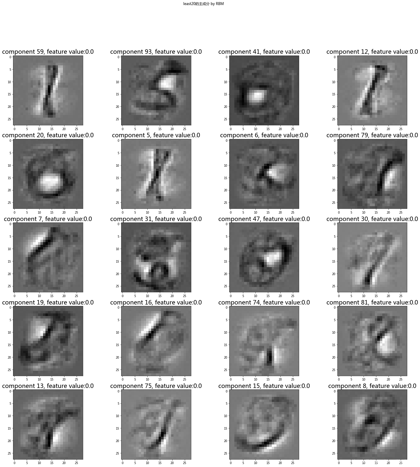
从上面看,59、12都不是表示lable=3的信息。
4. RBM在machine learning中效果
直接用LR模型
# import packages
from sklearn.linear_model import LogisticRegression
from sklearn.model_selection import GridSearchCV

# create LR
lr = LogisticRegression()
params = {'C':[1e-2, 1e-1, 1e0, 1e1, 1e2]}

# grid-search
grid = GridSearchCV(lr, params)
grid.fit(images_X, images_y)
GridSearchCV(cv=None, error_score='raise',
       estimator=LogisticRegression(C=1.0, class_weight=None, dual=False, fit_intercept=True,
          intercept_scaling=1, max_iter=100, multi_class='ovr', n_jobs=1,
          penalty='l2', random_state=None, solver='liblinear', tol=0.0001,
          verbose=0, warm_start=False),
       fit_params=None, iid=True, n_jobs=1,
       param_grid={'C': [0.01, 0.1, 1.0, 10.0, 100.0]},
       pre_dispatch='2*n_jobs', refit=True, return_train_score=True,
       scoring=None, verbose=0)
grid.best_estimator_, grid.best_score_
(LogisticRegression(C=0.1, class_weight=None, dual=False, fit_intercept=True,
           intercept_scaling=1, max_iter=100, multi_class='ovr', n_jobs=1,
           penalty='l2', random_state=None, solver='liblinear', tol=0.0001,
           verbose=0, warm_start=False), 0.88566666666666671)
采用PCA主成分的LR
lr = LogisticRegression()
pca = PCA()
params = {'clf__C':[1e-1, 1e0, 1e1], 'pca__n_components':[10, 100, 200]}
piplines = Pipeline([('pca', pca), ('clf', lr)])
grid_pca = GridSearchCV(piplines, params)
grid_pca.fit(images_X, images_y)
GridSearchCV(cv=None, error_score='raise',
       estimator=Pipeline(memory=None,
     steps=[('pca', PCA(copy=True, iterated_power='auto', n_components=None, random_state=None,
  svd_solver='auto', tol=0.0, whiten=False)), ('clf', LogisticRegression(C=1.0, class_weight=None, dual=False, fit_intercept=True,
          intercept_scaling=1, max_iter=100, multi_class='ovr', n_jobs=1,
          penalty='l2', random_state=None, solver='liblinear', tol=0.0001,
          verbose=0, warm_start=False))]),
       fit_params=None, iid=True, n_jobs=1,
       param_grid={'clf__C': [0.1, 1.0, 10.0], 'pca__n_components': [10, 100, 200]},
       pre_dispatch='2*n_jobs', refit=True, return_train_score=True,
       scoring=None, verbose=0)
grid_pca.best_estimator_, grid_pca.best_params_,grid_pca.best_score_
(Pipeline(memory=None,
      steps=[('pca', PCA(copy=True, iterated_power='auto', n_components=100, random_state=None,
   svd_solver='auto', tol=0.0, whiten=False)), ('clf', LogisticRegression(C=1.0, class_weight=None, dual=False, fit_intercept=True,
           intercept_scaling=1, max_iter=100, multi_class='ovr', n_jobs=1,
           penalty='l2', random_state=None, solver='liblinear', tol=0.0001,
           verbose=0, warm_start=False))]),
 {'clf__C': 1.0, 'pca__n_components': 100},
 0.88283333333333336)
pca的方法并未带来性能改善。
采用RBM主成分的LR
rbm = BernoulliRBM(random_state=0)
params = {'clf__C':[1e-1,1e0, 1e1], 'rbm__n_components':[10, 100, 200]}
pipeline = Pipeline([('rbm',rbm), ('clf',lr)])
grid_rbm = GridSearchCV(pipeline, params)
grid_rbm.fit(images_X, images_y)
GridSearchCV(cv=None, error_score='raise',
       estimator=Pipeline(memory=None,
     steps=[('rbm', BernoulliRBM(batch_size=10, learning_rate=0.1, n_components=256, n_iter=10,
       random_state=0, verbose=0)), ('clf', LogisticRegression(C=1.0, class_weight=None, dual=False, fit_intercept=True,
          intercept_scaling=1, max_iter=100, multi_class='ovr', n_jobs=1,
          penalty='l2', random_state=None, solver='liblinear', tol=0.0001,
          verbose=0, warm_start=False))]),
       fit_params=None, iid=True, n_jobs=1,
       param_grid={'clf__C': [0.1, 1.0, 10.0], 'rbm__n_components': [10, 100, 200]},
       pre_dispatch='2*n_jobs', refit=True, return_train_score=True,
       scoring=None, verbose=0)
grid_rbm.best_params_, grid_rbm.best_score_
({'clf__C': 1.0, 'rbm__n_components': 200}, 0.91266666666666663)
对比结果表明,RBM提高了LR的性能。
rbm = BernoulliRBM(random_state=0)
params = {'clf__C':[1e0], 'rbm__n_components':[200,300]}
pipeline = Pipeline([('rbm',rbm), ('clf',lr)])
grid_rbm2 = GridSearchCV(pipeline, params)
grid_rbm2.fit(images_X, images_y)
GridSearchCV(cv=None, error_score='raise',
       estimator=Pipeline(memory=None,
     steps=[('rbm', BernoulliRBM(batch_size=10, learning_rate=0.1, n_components=256, n_iter=10,
       random_state=0, verbose=0)), ('clf', LogisticRegression(C=1.0, class_weight=None, dual=False, fit_intercept=True,
          intercept_scaling=1, max_iter=100, multi_class='ovr', n_jobs=1,
          penalty='l2', random_state=None, solver='liblinear', tol=0.0001,
          verbose=0, warm_start=False))]),
       fit_params=None, iid=True, n_jobs=1,
       param_grid={'clf__C': [1.0], 'rbm__n_components': [200, 300]},
       pre_dispatch='2*n_jobs', refit=True, return_train_score=True,
       scoring=None, verbose=0)
grid_rbm2.best_params_, grid_rbm2.best_score_
({'clf__C': 1.0, 'rbm__n_components': 300}, 0.92016666666666669)
从上一会的结果看,RBM的components数量是200,意味着可以再考虑>200的参数。故在上面试验了采用300的参数,结果表明采用300的参数的LR性能更优。