边缘检测部分(各算子的内核未写明):
Sobel算子
Sobel算子是一个主要用于边缘检测的离散微分算子。
Sobel()
void cv::Sobel	(
InputArray 	src,
OutputArray 	dst,
int 	ddepth,
int 	dx,
int 	dy,
int 	ksize = 3,
double 	scale = 1,
double 	delta = 0,
int 	borderType = BORDER_DEFAULT
)
Parameters
src input image.
dst output image of the same size and the same number of channels as src .
ddepth output image depth, see combinations; in the case of 8-bit input images it will result in truncated derivatives.
图像输出的深度,输入输出组合见下表。需要注意的是当出入图像深度是8位时,会出现导数的截断。
dx order of the derivative x. X方向的导数
dy order of the derivative y. Y方向的导数
ksize size of the extended Sobel kernel; it must be 1, 3, 5, or 7. Sobel算子的核心,其宽度必须是奇数。
scale optional scale factor for the computed derivative values; by default, no scaling is applied . 计算导数时可选的缩放因子,默认不缩放。
delta optional delta value that is added to the results prior to storing them in dst.输出dst之前可选的值,默认值为0.
borderType pixel extrapolation method, see cv::BorderTypes.边缘类型

简单介绍一下:
Sobel算子包含任意阶的微分以及融合偏导。
计算图像X方向的导数【xorder=0,yorder=1,ksize=3】,计算图像Y方向的导数【xorder=1,yorder=0,ksize=3】。
xorder和yorder是求导的阶数。通常只用到0、1,最多2。
ksize是方形滤波器的宽并且应该是奇数。
如果源图像是8位的,为避免溢出,目标图像的深度必须是CV_16S。
Sobel导数有一个非常好的性质,即可以定义任意大小的核,并且这些核可以用快速且迭代的方式构造。大核对导数有更好的逼近,因为小核对噪声更敏感。
Sobel导数并不是真正意义上的导数,因为Sobel算子定义于一个离散的空间之上。Sobel算子真正表示的是多项式拟合,也就是说,x方向上的二阶Sobel导数并不是真正的二阶导数。它是对抛物线函数的局部拟合。正因此,较大的核可以在更多像素上进行覆盖,从而达到更好的拟合效果。
Sobel算子的效果演示:
#include <opencv2\opencv.hpp>
#include <opencv2\highgui\highgui.hpp>
#include <opencv2\imgproc\imgproc.hpp>
using namespace cv;

int main()
{
	Mat grad_x, grad_y;
	Mat abs_grad_x, abs_grad_y, dst;

	Mat src = imread("1.png");
	cvtColor(src, src, COLOR_BGR2GRAY);//输出8位图
	imshow("原始图", src);

	Sobel(src, grad_x, CV_16S, 1, 0, 3, 1, 0, BORDER_DEFAULT);
	convertScaleAbs(grad_x, abs_grad_x);//转换成8位无符号
	imshow("效果图1", abs_grad_x);//x方向

	Sobel(src, grad_y, CV_16S, 0, 1, 3, 1, 1, BORDER_DEFAULT);
	convertScaleAbs(grad_y, abs_grad_y);
	imshow("效果图2", abs_grad_y);

	addWeighted(abs_grad_x, 0.5, abs_grad_y, 0.5, 0, dst);
	imshow("效果图3", dst);//两个方向融合

	waitKey();
	destroyAllWindows();
	return 0;

}


Scharr滤波器
上面已经提到,对于小一点的核而言,这种使用Sobel算子近似计导数的缺点是精确度较低。对于大核,由于在估计时使用了更多的点,所以这个问题并不严重。对于一个3x3的Sobel滤波器,当梯度角度越接近水平或垂直方向时,这种不准确就更加明显。
Scharr滤波器同Sobel滤波器一样快,但准确度更高,所以当你利用3x3滤波器实现图像度量的时候应该使用Scharr滤波器。
◆ Scharr()
void cv::Scharr	(	InputArray 	src,
OutputArray 	dst,
int 	ddepth,
int 	dx,
int 	dy,
double 	scale = 1,
double 	delta = 0,
int 	borderType = BORDER_DEFAULT
)
当计算水平方向和垂直方向的一阶微分时,使用Scharr滤波器。
Parameters
src input image.
dst output image of the same size and the same number of channels as src.
ddepth output image depth, see combinations
dx order of the derivative x.
dy order of the derivative y.
scale optional scale factor for the computed derivative values; by default, no scaling is applied (see getDerivKernels for details).
delta optional delta value that is added to the results prior to storing them in dst.
borderType pixel extrapolation method, see cv::BorderTypes
Scharr滤波器效果:
#include <opencv2\opencv.hpp>
#include <opencv2\highgui\highgui.hpp>
#include <opencv2\imgproc\imgproc.hpp>
using namespace cv;

int main()
{
	Mat grad_x, grad_y;
	Mat abs_grad_x, abs_grad_y, dst;

	Mat src = imread("1.png");
	cvtColor(src, src, COLOR_BGR2GRAY);
	imshow("原始图", src);

	Sobel(src, grad_x, CV_16S, 1, 0, 3, 1, 0, BORDER_DEFAULT);
	convertScaleAbs(grad_x, abs_grad_x);//转换成8位无符号
	imshow("效果图1", abs_grad_x);

	Sobel(src, grad_y, CV_16S, 0, 1, 3, 1, 1, BORDER_DEFAULT);
	convertScaleAbs(grad_y, abs_grad_y);
	imshow("效果图2", abs_grad_y);

	addWeighted(abs_grad_x, 0.5, abs_grad_y, 0.5, 0, dst);
	imshow("效果图3", dst);

	waitKey();
	destroyAllWindows();
	return 0;

}


可与上面的Sobel算子进行对比,同样是3x3的内核,在水平方形与垂直方向Scharr滤波器细节更加丰富。
对于一阶微分算子,也就是一阶导数,对于一个函数(连续)而言代表的是其斜率(假设只考虑大于0),对于一副图像,当这个图像的像素值一直增大然后再减小,极值位于一阶微分等于0处,在这个点取得的像素其实更好地代表了像素的变化边界,所以一阶微分是能检测出边缘的。
Laplacian算子
拉普拉斯算子的输出形式:

因为拉普拉斯算子可以用二次导数的形式定义,可假设其离散实现类似于二阶Sobel导数,事实也确实如此,OpenCV在计算拉普拉斯算子时直接使用Sobel算子。
◆ Laplacian()
void cv::Laplacian	(	InputArray 	src,
OutputArray 	dst,
int 	ddepth,
int 	ksize = 1,
double 	scale = 1,
double 	delta = 0,
int 	borderType = BORDER_DEFAULT
)
Parameters
src Source image.
dst Destination image of the same size and the same number of channels as src .
ddepth Desired depth of the destination image.
ksize Aperture size used to compute the second-derivative filters. See getDerivKernels for details. The size must be positive and odd.
scale Optional scale factor for the computed Laplacian values. By default, no scaling is applied. See getDerivKernels for details.
delta Optional delta value that is added to the results prior to storing them in dst .
borderType Pixel extrapolation method, see cv::BorderTypes
对于拉普拉斯函数,当我们逼近类似边缘的不连续地方导数会快速增长,而穿过这些不连续的地方时导数又会快速减小。所以导数在此范围内有局部极值。这样原始图像的边缘位于拉普拉斯的值等于0的地方。
对于一个高次曲线,二阶微分等于0对应的是它的拐点,位于拐点两边的函数凹凸性是不一样的,也就是说在拐点的两边分别是像素值增大或者减小的一种,从而拐点就很好的标识了一副图像的边界区域。
Laplacian算子演示:
#include <opencv2\opencv.hpp>
#include <opencv2\highgui\highgui.hpp>
#include <opencv2\imgproc\imgproc.hpp>
using namespace cv;

int main()
{
	Mat src, src_gray, dst, abs_dst;

	src = imread("1.png");

	imshow("原图", src);

	GaussianBlur(src, src, Size(3, 3), 0, 0, BORDER_DEFAULT);

	cvtColor(src, src_gray, COLOR_RGB2GRAY);

	Laplacian(src_gray, dst, CV_16S, 3, 1, 0, BORDER_DEFAULT);

	convertScaleAbs(dst, abs_dst);

	imshow("效果图", abs_dst);
	waitKey();
	destroyAllWindows();
	return 0;
}

注:让一副图像减去它的Laplacian算子可以增强对比度。

Canny算子
Canny算法和拉普拉斯算法不同点之一是在Canny算法中,首先在x和y方向求一阶导数,然后组合为4个方向的导数。这些方向导数达到局部最大值的点就是组成边缘的候选点。Canny算法最重要的一个新特点是其试图将独立边的候选像素拼装成轮廓。其使用了滞后性阈值,分别为上、下两个阈值。如果一个像素的梯度大于上限阈值,则被认为是边缘像素,如果低于下限阈值,则被抛弃,如果介于二者之间,只有当其与高于上限阈值的像素连接时才会被接受。Canny土建的上下限阈值比为2:1到3:1之间。
◆ Canny() [2/2]
void cv::Canny	(	InputArray 	dx,
InputArray 	dy,
OutputArray 	edges,
double 	threshold1,
double 	threshold2,
bool 	L2gradient = false
)
Parameters
image 8-bit input image.
edges output edge map; single channels 8-bit image, which has the same size as image .
threshold1 first threshold for the hysteresis procedure.
threshold2 second threshold for the hysteresis procedure.
apertureSize aperture size for the Sobel operator.
L2gradient a flag, 计算图像梯度幅值的标识,默认值为false。
注意:Canny算子的输入输出的图形必须为灰度图像。
Canny算子演示:
#include <opencv2\opencv.hpp>
#include <opencv2\highgui\highgui.hpp>
#include <opencv2\imgproc\imgproc.hpp>
using namespace cv;

int main()
{
	Mat src = imread("1.png");
	Mat src1 = src.clone();
	imshow("原图", src);
	//opencv3中不能直接调用Canny函数,需要进行要预处理

	Mat dst, edge, gray;

	dst.create(src1.size(), src1.type());//创建于src1同类型和大小的dst

	cvtColor(src1, gray, COLOR_BGR2GRAY);

	blur(gray, edge, Size(3, 3));//降噪

	Canny(edge, edge, 3, 3);

	imshow("效果图1", edge);

	dst = Scalar::all(0);

	src1.copyTo(dst, edge);
	imshow("效果图2", dst);

	waitKey(0);
	destroyAllWindows();
	return 0;


}

霍夫变换(Hough Transform)
霍夫变换是一种在图像中寻找直线,圆及其他简单形状的方法。
霍夫线变换
霍夫直线变换的基本理论是二值图像中的任何点都可能是一些候选直线集合的一部分。霍夫线变换的输入图像只能是边缘二值图像,所以在进行变换之前要对原始图像进行边缘检测处理。
原理:
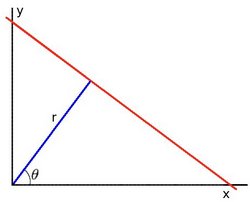
霍夫直线变换目的在于找出处于同一直线上的点,然后将他们绘制出来,这样就会形成一条直线。采用(x,y)难以将多条直线简单的标识出来,而采用(r,θ)可以将直线描绘成坐标系中的一个点。
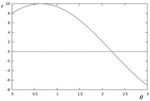
由直角坐标系中的图像可以得到。如给定一个点(x0,y0),绘制出所有通过它的直线能打得到类似正弦函数的一张图像,当对多个点进行同时绘制,就会得到多条图像。当给定多个点进行绘制,如果多条曲线经过一个点(极坐标中交点代表的是直线),那么说明这些给定的点都在同一条直线上。
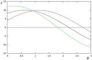
那么越多曲线交于一点就代表着经过(交点处所代表的直线)的点越多。由此,通过设置一个阈值来定义多少条曲线交于一点,来判断这些点是否在一条直线上。
标准霍夫变换:HoughLines()函数
◆ HoughLines()
void cv::HoughLines	(	InputArray 	image,
OutputArray 	lines,
double 	rho,
double 	theta,
int 	threshold,
double 	srn = 0,
double 	stn = 0,
double 	min_theta = 0,
double 	max_theta = CV_PI
)
该函数的功能是同过标准霍夫变换在二值图像中找出直线。
Parameters(参数):
image 8-bit, single-channel binary source image. The image may be modified by the function.输入图像8位单通道二值图像
lines Output vector of lines. Each line is represented by a two-element vector (ρ,θ) . ρ is the distance from the coordinate origin (0,0) (top-left corner of the image). θ is the line rotation angle in radians ( 0∼vertical line,π/2∼horizontal line ).
输出的是向量,每一条直线由该二维向量的(ρ,θ)指定,ρ 是极径,θ是极角。
rho Distance resolution of the accumulator in pixels.在累加器中的点之间的距离,以像素为单位。
theta Angle resolution of the accumulator in radians.在累加器中的点之间的角度,以弧度为单位。
threshold Accumulator threshold parameter. Only those lines are returned that get enough votes ( >threshold ).
累加器中的阈值,即识别某部分为图中一条直线时它在累加器中必须达到的值。
srn For the multi-scale Hough transform, it is a divisor for the distance resolution rho . The coarse accumulator distance resolution is rho and the accurate accumulator resolution is rho/srn . If both srn=0 and stn=0 , the classical Hough transform is used. Otherwise, both these parameters should be positive.对于多尺度霍夫变换,它是距离分辨率rho的除数。有默认值0
stn For the multi-scale Hough transform, it is a divisor for the distance resolution theta.
min_theta For standard and multi-scale Hough transform, minimum angle to check for lines. Must fall between 0 and max_theta.
max_theta For standard and multi-scale Hough transform, maximum angle to check for lines. Must fall between min_theta and CV_PI.
程序实例:
#include <opencv2\opencv.hpp>
#include <opencv2\imgproc\imgproc.hpp>
using namespace std;
using namespace cv;

int main()
{
	Mat srcImage = imread("1.jpg");
	Mat midImage, dstimage;

	Canny(srcImage, midImage, 50, 200, 3);
	cvtColor(midImage, dstimage, CV_GRAY2BGR);
	vector<Vec2f> lines;
	HoughLines(midImage, lines, 1, CV_PI / 180, 100, 0, 0);

	for (int  i = 0; i < lines.size(); i++)
	{
		float rho = lines[i][0], theta = lines[i][1];
		Point pt1, pt2;
		double a = cos(theta), b = sin(theta);
		double x0 = a*rho, y0 = b*rho;
		pt1.x = cvRound(x0 + 1000 * (-b));
		pt1.y = cvRound(y0 + 1000 * (a));
		pt2.x = cvRound(x0 - 1000 * (-b));
		pt2.y = cvRound(y0 - 1000 * (a));
		line(dstimage, pt1, pt2, Scalar(55, 100, 195), 1, LINE_AA);

	}
	imshow("原图", srcImage);
	imshow("边缘检测", midImage);
	imshow("直线检测", dstimage);
	waitKey();
	destroyAllWindows();
	return 0;
}
注:程序中的1000是为了给定将要绘制直线的起始点和终点,霍夫线变换可以知道直线中的点,但无法确定哪里是线段的起点和终点。程序中找出了给定点上方1000距离的点和下方1000距离的点作为起始点和终点。可根据具体情况设定其他值。


累计概率霍夫变换:HoughLinesP()
此函数在HougLines的基础上,在末尾加了一个P表示累计概率霍夫变换(PPHT)。
◆ HoughLinesP()
void cv::HoughLinesP	(	InputArray 	image,
OutputArray 	lines,
double 	rho,
double 	theta,
int 	threshold,
double 	minLineLength = 0,
double 	maxLineGap = 0
)
该函数用于找出图像中的线段。PPHT是标准霍夫变换(SHT)的一个变种,计算单独线段的方向以及范围。
Parameters
image 8-bit, single-channel binary source image. The image may be modified by the function.
lines Output vector of lines. Each line is represented by a 4-element vector (x1,y1,x2,y2) , where (x1,y1) and (x2,y2) are the ending points of each detected line segment.
rho Distance resolution of the accumulator in pixels.
theta Angle resolution of the accumulator in radians.
threshold Accumulator threshold parameter. Only those lines are returned that get enough votes ( >threshold ).
minLineLength Minimum line length. Line segments shorter than that are rejected.返回最小线段长度。
maxLineGap Maximum allowed gap between points on the same line to link them.设置为一条直线上分离线段不能连成一条直线的分割像素点数。
程序示例:
#include <opencv2\opencv.hpp>
#include <opencv2\imgproc\imgproc.hpp>
using namespace cv;
using namespace std;

int main()
{
	Mat srcImage = imread("1.jpg");
	Mat midImage, dstIamge;

	Canny(srcImage, midImage, 50, 200, 3);
	cvtColor(midImage, dstIamge, CV_GRAY2BGR);
	vector<Vec4i> lines;
	HoughLinesP(midImage, lines, 1, CV_PI / 180, 80, 50, 5);

	for (size_t i = 0; i < lines.size(); i++)
	{
		Vec4i l = lines[i];
		line(dstIamge, Point(l[0], l[1]), Point(l[2], l[3]), Scalar(0, 255, 255), 1, LINE_AA);
		imshow("原始图", srcImage);
		imshow("边缘检测后的图", midImage);
		imshow("直线检测后的图", dstIamge);
	}
	waitKey();
	destroyAllWindows();
	return 0;
}
霍夫圆变换
◆ HoughCircles()
void cv::HoughCircles	(	InputArray 	image,
OutputArray 	circles,
int 	method,
double 	dp,
double 	minDist,
double 	param1 = 100,
double 	param2 = 100,
int 	minRadius = 0,
int 	maxRadius = 0
)
霍夫圆变换能很好地找出圆心,对于半径有时候可能无法正确找到。
Parameters
image 8-bit, single-channel, grayscale input image.
circles Output vector of found circles. Each vector is encoded as a 3-element floating-point vector (x,y,radius) .
method Detection method, see cv::HoughModes. Currently, the only implemented method is HOUGH_GRADIENT
dp Inverse ratio of the accumulator resolution to the image resolution. For example, if dp=1 , the accumulator has the same resolution as the input image. If dp=2 , the accumulator has half as big width and height.
minDist Minimum distance between the centers of the detected circles. If the parameter is too small, multiple neighbor circles may be falsely detected in addition to a true one. If it is too large, some circles may be missed.
param1 First method-specific parameter. In case of CV_HOUGH_GRADIENT , it is the higher threshold of the two passed to the Canny edge detector (the lower one is twice smaller).
param2 Second method-specific parameter. In case of CV_HOUGH_GRADIENT , it is the accumulator threshold for the circle centers at the detection stage. The smaller it is, the more false circles may be detected. Circles, corresponding to the larger accumulator values, will be returned first.
minRadius Minimum circle radius.
maxRadius Maximum circle radius.
程序示例:
#include <opencv2\opencv.hpp>
#include <opencv2\imgproc\imgproc.hpp>
using namespace std;
using namespace cv;

int main()
{
	Mat srcImage = imread("1.jpg");
	Mat midImage, dstImage;

	imshow("原始图", srcImage);

	cvtColor(srcImage, midImage, COLOR_BGR2GRAY);
	GaussianBlur(midImage, midImage, Size(9, 9), 2, 2);
	vector<Vec3f> circles;
	HoughCircles(midImage, circles, HOUGH_GRADIENT, 2, 30, 100, 100, 0, 0);
	for (size_t i = 0; i < circles.size(); i++)
	{
		Point center(cvRound(circles[i][0]), cvRound(circles[i][1]));
		int radius = cvRound(circles[i][2]);
		circle(srcImage, center, 3, Scalar(0, 255, 0), -1, 8, 0);
		circle(srcImage, center, radius, Scalar(0, 0, 0), 3, 8, 0);
	}
	imshow("效果图", srcImage);
	waitKey();
	destroyAllWindows();
	return 0;
}
重映射
重映射其实就是把一副图像中的像素放置到另一个图像中的指定位置以实现图像变换。
实现重映射的函数:remap()
◆ remap()
void cv::remap	(	InputArray 	src,
OutputArray 	dst,
InputArray 	map1,
InputArray 	map2,
int 	interpolation,
int 	borderMode = BORDER_CONSTANT,
const Scalar & 	borderValue = Scalar()
)
该函数不支持就地操作。
Parameters
src Source image.
dst Destination image. It has the same size as map1 and the same type as src .
map1 The first map of either (x,y) points or just x values having the type CV_16SC2 , CV_32FC1, or CV_32FC2. See convertMaps for details on converting a floating point representation to fixed-point for speed.
map1表示两种情况,第一种表示点(x,y)的一个映射,只映射一个点;第二种情况表示具有CV_16SC2 , CV_32FC1, or CV_32FC2类型的X值。
map2 The second map of y values having the type CV_16UC1, CV_32FC1, or none (empty map if map1 is (x,y) points), respectively.
对于map2 ,当map1表示一个点时,无意义;否则就表示CV_16SC2 , CV_32FC1的Y值。
interpolation Interpolation method (see cv::InterpolationFlags). The method INTER_AREA is not supported by this function.
插值, INTER_AREA 在该函数中无法使用。
常用插值:
INTER_NEAREST
Python: cv.INTER_NEAREST
nearest neighbor interpolation
INTER_LINEAR
Python: cv.INTER_LINEAR
bilinear interpolation
INTER_CUBIC
Python: cv.INTER_CUBIC
borderMode Pixel extrapolation method (see cv::BorderTypes). When borderMode=BORDER_TRANSPARENT, it means that the pixels in the destination image that corresponds to the "outliers" in the source image are not modified by the function.
边界模式,默认值为BORDER_CONSTANT。
borderValue Value used in case of a constant border. By default, it is 0.
简单的来说,重映射就是改变原图像中的像素点的位置,然后保存到另一幅图像中,通常从X和Y两个方向改变。
代码示例:
#include <opencv2/highgui/highgui.hpp>
#include <opencv2\imgproc\imgproc.hpp>
#include <iostream>
using namespace std;
using namespace cv;

#define WINDOW_NAME "程序窗口"

Mat g_srcImage, g_dstImage;
Mat g_map_x, g_map_y;//定义X和Y方向的像素矩阵,用于保存改变位置后的像素。

int update_map(int key);
static void ShowHelpText();
int main()
{
	system("color 2F");
	ShowHelpText();
	g_srcImage = imread("1.jpg");//读取图像
	if (!g_srcImage.data)
	{
		printf("error!");
		return false;
	}
	imshow("原图", g_srcImage);
	g_dstImage.create(g_srcImage.size(), g_srcImage.type());
	g_map_x.create(g_srcImage.size(), CV_32FC1);//分配x方向的矩阵空间和类型
	g_map_y.create(g_srcImage.size(), CV_32FC1);

	namedWindow(WINDOW_NAME, WINDOW_AUTOSIZE);
	imshow(WINDOW_NAME, g_srcImage);
	while (1)
	{
		int key = waitKey(0);
		if ((key & 255) == 27)
		{
			cout << "程序退出.." << endl;
			break;
		}
		update_map(key);
		remap(g_srcImage, g_dstImage, g_map_x, g_map_y, INTER_LINEAR, BORDER_CONSTANT, Scalar(0, 0, 0));
		imshow(WINDOW_NAME, g_dstImage);

	}

	destroyAllWindows();
	return 0;
}

int update_map(int key)
{
	for (int j = 0; j < g_srcImage.rows; j++)
	{
		for (int i = 0; i < g_srcImage.cols; i++)
		{
			switch (key)
			{
			case '1'://显示图像的中间部分,距离上下左右四分之一的距离
				if (i > g_srcImage.cols*0.25&&i<g_srcImage.cols*0.75&&
					j>g_srcImage.rows*0.25&&j < g_srcImage.rows*0.75)
				{
					g_map_x.at<float>(j, i) = static_cast<float>(2 * (i - g_srcImage.cols*0.25) + 0.5);
					g_map_y.at<float>(j, i) = static_cast<float>(2 * (j - g_srcImage.rows*0.25) + 0.5);

				}

				break;
			case '2':
				g_map_x.at<float>(j, i) = static_cast<float>(i);//翻转Y方向的像素值
				g_map_y.at<float>(j, i) = static_cast<float>(g_srcImage.rows - j);
				break;
			case '3':
				g_map_x.at<float>(j, i) = static_cast<float>(g_srcImage.cols - i);
				g_map_y.at<float>(j, i) = static_cast<float>(j);
				break;
			case '4':
				g_map_x.at<float>(j, i) = static_cast<float>(g_srcImage.cols - i);
				g_map_y.at<float>(j, i) = static_cast<float>(g_srcImage.rows - j);
				break;
			}
		}
	}
	return 1;

}
static void ShowHelpText()
{
	printf("欢迎来到重映射示例程序\n");

}

仿射变换
重映射在于将图像中的像素重新排列,不管有没有意义,像素间的相对位置一般都会改变。
放射变换目的在于保持像素相对位置不变的情况下对图像进行位置上的改变,比如旋转,平移,缩放等。
放射变换中的变换矩阵:对一整幅图像进行操作实际上就是对图像中所有的像素点进行相同的操作,在计算机图形学中经常把平面上的点进行平移、旋转、缩放等操作。对于单个的点可以看成行(列)向量,而对于一副图像就是一个矩阵。同样的变换后的图像一样是一个矩阵。那么,当一个矩阵乘上一个矩阵变成了另一个矩阵(假设都是可逆矩阵),那么就可以根据矩阵的运算计算出乘上的这个矩阵,也就是变换矩阵。有了变换矩阵,即使源图像不一样,也可以得到想要的结果了。
获得变换矩阵:getAffineTransform()
getAffineTransform() [1/2]
Mat cv::getAffineTransform	(
const Point2f 	src[],
const Point2f 	dst[]
)
该函数用于从三对对应点得到变换矩阵,即在输入的三个点和输出的三个点之间计算出变换矩阵。
Parameters
src Coordinates of triangle vertices in the source image.
dst Coordinates of the corresponding triangle vertices in the destination image.
进行仿射变换:warpAffine()
◆ warpAffine()
void cv::warpAffine	(	InputArray 	src,
OutputArray 	dst,
InputArray 	M,
Size 	dsize,
int 	flags = INTER_LINEAR,
int 	borderMode = BORDER_CONSTANT,
const Scalar & 	borderValue = Scalar()
)
Parameters
src input image.
dst output image that has the size dsize and the same type as src .
M 2×3 transformation matrix.尺寸为2x3的变换矩阵。
dsize size of the output image.
flags combination of interpolation methods (see cv::InterpolationFlags) and the optional flag WARP_INVERSE_MAP that means that M is the inverse transformation ( dst→src ).插值方式。
borderMode pixel extrapolation method (see cv::BorderTypes); when borderMode=BORDER_TRANSPARENT, it means that the pixels in the destination image corresponding to the "outliers" in the source image are not modified by the function.
borderValue value used in case of a constant border; by default, it is 0.
进行二维旋转变换:getRotationMatrix2D()
◆ getRotationMatrix2D()
Mat cv::getRotationMatrix2D	(	Point2f 	center,
double 	angle,
double 	scale
)
该函数用于计算二维旋转变换矩阵。旋转变换根据角度可计算出其相应的变换矩阵,沿逆时针方向旋转为正角度。
Parameters
center Center of the rotation in the source image.旋转中心的坐标
angle Rotation angle in degrees. Positive values mean counter-clockwise rotation (the coordinate origin is assumed to be the top-left corner).旋转角。
scale Isotropic scale factor.缩放系数。
程序示例:
#include <opencv2\opencv.hpp>
#include <opencv2\imgproc\imgproc.hpp>
#include <iostream>
using namespace std;
using namespace cv;

#define WINDOW_NAME1 "原始窗口"
#define WINDOW_NAME2 "Warp后的图像"
#define WINDOW_NAME3 "Warp和Rotate后的图像"


int main()
{
	system("color 1A");

	Point2f srcTriangle[3];
	Point2f dstTriangle[3];

	Mat rotMat(2, 3, CV_32FC1);
	Mat warpMat(2, 3, CV_32FC1);
	Mat srcImage, dstImage_warp, dstImage_warp_rotate;
	srcImage = imread("1.jpg");
	if (!srcImage.data)
	{
		printf("error!");
		return false;
	}
		dstImage_warp.create(srcImage.size(), srcImage.type());
		//设置初始点
		srcTriangle[0] = Point2f(0, 0);//左上角的点
		srcTriangle[1] = Point2f(static_cast<float>(srcImage.cols - 1),0);//右上角的点
		srcTriangle[2] = Point2f(0,static_cast<float>(srcImage.rows - 1));//左下角的点
		//设置对应的三个结果点
		dstTriangle[0] = Point2f(static_cast<float>(srcImage.cols*0.0),
			static_cast<float>(srcImage.rows*0.33));
		dstTriangle[1] = Point2f(static_cast<float>(srcImage.cols*0.65),
			static_cast<float>(srcImage.rows*0.35));
		dstTriangle[2] = Point2f(static_cast<float>(srcImage.cols*0.15),
			static_cast<float>(srcImage.rows*0.6));

		//求得变换矩阵
		warpMat = getAffineTransform(srcTriangle, dstTriangle);
		//进行仿射变换
		warpAffine(srcImage, dstImage_warp, warpMat, dstImage_warp.size());
		Point center = Point(dstImage_warp.cols / 2, dstImage_warp.rows / 2);//设置旋转变换的中心点
		double angle = -30.0;//顺时针旋转
		double scale = 0.8;//缩小为原来的0.8倍
		rotMat = getRotationMatrix2D(center, angle, scale);//旋转
		warpAffine(dstImage_warp, dstImage_warp_rotate, rotMat, dstImage_warp.size());
		imshow(WINDOW_NAME1, srcImage);//源图像
		imshow(WINDOW_NAME2, dstImage_warp);//仿射变换的图像
		imshow(WINDOW_NAME3, dstImage_warp_rotate);//仿射变换后进行旋转的图像
		waitKey();
		destroyAllWindows();
		return 0;

}

直方图均衡化
直方图均衡化是灰度变换的一个重要应用,广泛应用与图像增强处理中,是通过拉伸像素强度分布范围来增强图像对比度的一种方法。
实现直方图均衡化:equalizeHist()
◆ equalizeHist()
void cv::equalizeHist	(	InputArray 	src,
OutputArray 	dst
)
程序示例:
#include <opencv2\highgui\highgui.hpp>
#include <opencv2\imgproc\imgproc.hpp>
using namespace cv;

int main()
{
	Mat srcImage, dstImage;
	srcImage = imread("1.jpg", 1);
	if (!srcImage.data)
	{
		printf("error!");
		return false;
	}
	cvtColor(srcImage, srcImage, CV_BGR2GRAY);
	imshow("原始图", srcImage);

	equalizeHist(srcImage, dstImage);
	imshow("经过直方图均衡化后的图", dstImage);
	waitKey();
	destroyAllWindows();
	return 0;
}
