OpenCV 直方图均衡化
对曝光过度或者逆光拍摄的图片可以通过直方图均衡化的方法用来增强局部或者整体的对比度。
具体思路是通过找出图像中最亮和最暗的像素值将之映射到纯黑和纯白之后再将其他的像素值按某种算法映射到纯黑和纯白之间的值。另一种方法是寻找图像中像素的平均值作为中间灰度值,然后扩展范围以达到尽量充满可显示的值。
直方图
什么是直方图?你可以把直方图看作一个图或图,它给你一个关于图像的强度分布的总体思路。它是一个带有像素值的图(从0到255,不总是)在x轴上,在y轴上的图像对应的像素个数。
这只是理解图像的另一种方式。通过观察图像的直方图,你可以直观地了解图像的对比度、亮度、亮度分布等。今天几乎所有的图像处理工具都提供了直方图上的特征。以下是来自Cambridge in Color website的图片,建议去访问这个网站,了解更多细节。
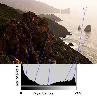
你可以看到图像和它的直方图。(这个直方图是用灰度图像绘制的,而不是彩色图像)。直方图的左边部分显示了图像中较暗像素的数量,右边区域显示了更明亮的像素。从直方图中可以看到,深色区域的像素数量比亮色区域更多,而中间色调的数量(中值大约在127左右)则少得多。
直方图相关术语
现在我们已经知道了什么是直方图,我们可以看看如何得到它。OpenCV和Numpy都有内置的功能。在使用这些函数之前,我们需要了解一些与直方图相关的术语。
BINS
BINS:上面的直方图显示了每个像素值的像素数,从0到255。您需要256个值来显示以上的直方图。但是,考虑一下,如果您不需要单独查找所有像素值的像素数量,而是在一个像素值区间内的像素数量,该怎么办?例如,你需要找到介于0到15之间的像素数,然后是16到31……240到255。您只需要16个值来表示这个直方图。OpenCV Tutorials on histograms中展示了这个例子。
所以你要做的就是把整个直方图分成16个子部分,每个子部分的值是所有像素数的和。每个子部分都被称为“BIN”。在第一种情况下,BINS的数量是256(每个像素一个),而在第二种情况下,它只有16个。在OpenCV文档中,用术语 histSize 表示 BINS。
DIMS
DIMS:它是我们收集数据的参数的个数。在这种情况下,我们收集的数据只有一件事,强度值。所以这里是1。
RANGE
RANGE:它是你想测量的强度值的范围。通常,它是 [ 0,256 ],也就是所有的强度值。
OpenCV中直方图的计算
OpenCV提供了cv.calcHist()函数来获取直方图。让我们熟悉一下这个函数及其参数:
cv.calcHist(images, channels, mask, histSize, ranges[, hist[, accumulate]])
- 1
images:它是uint8类型或float32的源图像。它应该用方括号括起来,也就是”[img]”。
channels:它也用方括号括起来。它是我们计算直方图的信道的索引。例如,如果输入是灰度图像,它的值是0。对于颜色图像,您可以通过0、1或2来分别计算蓝色、绿色或红色通道的直方图。
mask:遮罩图。为了找到完整图像的直方图,它被指定为“None”。但如果你想找到图像的特定区域的直方图,你必须为它创建一个遮罩图,并将其作为遮罩。
histSize:这代表了我们的BINS数。需要用方括号来表示。在整个范围内,我们通过了256。
ranges:强度值范围,通常是 [ 0,256 ]
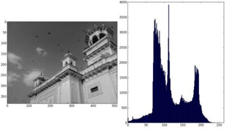
让我们从一个样本图像开始。只需在灰度模式下加载图像并找到其完整的直方图。
img = cv.imread('home.jpg', 0)
hist = cv.calcHist([img], [0], None, [256], [0,256])
- 1
- 2
hist是一个256x1阵列,每个值对应于该图像中的像素值及其对应的像素值。
Numpy中直方图的计算
Numpy中提供了np.histogram()方法,用于对一维数组进行直方图统计,其参数列表如下:
Histogram(a,bins=10,range=None,normed=False,weights=None)
- 1
a:是保存待统计的数组
bins:指定统计的区间个数,即对统计范围的等分数
range:是一个长度为2的元组,表示统计范围的最大值和最小值,默认值为None,表示范围由数据的范围决定,即(a.min(), a.max))。
normed:当normed参数为False时,函数返回数组a中的数据在每个区间的个数,否则对个数进行正规化处理,使它等于每个区间的概率密度。
weights:weights参数和 bincount()的类似
返回值,有两个,
hist : hist和之前计算的一样,每个区间的统计结果。
bins : 数组,存储每个统计区间的起点。range为[0,256]时,bins有257个元素,因为Numpy计算bins是以0-0.99,1-1.99等,所以最后一个是255-255.99。为了表示这一点,他们还在bins的末端添加了256。但我们不需要256。到255就足够了。
让我们从一个样本图像开始。只需在灰度模式下加载图像并找到其完整的直方图。
hist, bins = np.histogram(img.ravel(), 255, [0,256])
- 1
Numpy还有另一个函数,np.bincount(),比np.histograme()要快得多(大约10X)。对于一维直方图,你可以试一下。不要忘记在np.bincount中设置minlength=256。例如,hist=np.bincount(img.ravel(),minlength=256)
OpenCV函数比np.histogram()快(大约40X)。所以考虑效率的时候坚持用OpenCV函数。
绘制直方图
1. 使用Matplotlib
Matplotlib有一个绘制直方图的函数:
matplotlib.pyplot.hist()
- 1
它直接找到了直方图并绘制了它。您不需要使用calcHist()或np.histogram()函数来找到直方图。看下面的代码:
import numpy as np
import cv2 as cv
from matplotlib import pyplot as plt

img = cv.imread('home.jpg', 0)
plt.hist(img.ravel(), 256, [0,256])
plt.show()
- 1
- 2
- 3
- 4
- 5
- 6
- 7
或者你可以用常规的matplotlib的plot函数绘制直方图,适合绘制BGR图像直方图。为此,您需要首先找到直方图数据。试试下面的代码
import numpy as np
import cv2 as cv
from matplotlib import pyplot as plt

img = cv.imread('home.jpg')
color = ('b', 'g', 'r')
for i, col in enumerate(color):
    histr = cv.calcHist([img], [i], None, [256], [0,256])
    plt.plot(histr, color=col)
    plt.xlim([0,256])
plt.show()
- 1
- 2
- 3
- 4
- 5
- 6
- 7
- 8
- 9
- 10
- 11
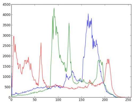
你可以从上面的图中看出,蓝色在图像中有一些高值区域(很明显,它应该是由天空引起的)
2. 使用OpenCV
你可以调整直方图的值和它的bin值,让它看起来像x,y坐标,这样你就可以用cv.line()或cv.polyline()函数来绘制它,从而生成与上面相同的图像。这已经是OpenCV-Python2官方的样本了。查看sampl/python/hist.py的代码。
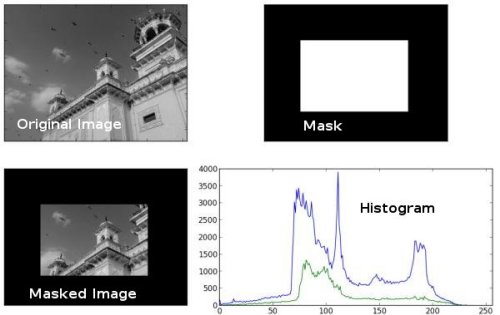
应用遮罩
我们用cv.calcHist()函数来找一张完整的图片的直方图。但是我们只要图片的一部分的直方图呢?在你想要找到的区域中,创建一个带有白色的遮罩图像。然后把它作为遮罩。
img = cv.imread('home.jpg', 0)

# create a mask
mask = np.zeros(img.shape[:2], np.uint8)
mask[100:300, 100:400] = 255
masked_img = cv.bitwise_and(img, img, mask=mask)

#Calculate histogram with mask and without mask
Check third argument for mask
hist_full = cv.calcHist([img], [0], None, [256], [0,256])
hist_mask = cv.calcHist([img], [0], mask, [256], [0,256])

plt.subplot(221), plt.imshow(img, 'gray')
plt.subplot(222), plt.imshow(mask,'gray')
plt.subplot(223), plt.imshow(masked_img, 'gray')
plt.subplot(224), plt.plot(hist_full), plt.plot(hist_mask)
plt.xlim([0,256])

plt.show()
- 1
- 2
- 3
- 4
- 5
- 6
- 7
- 8
- 9
- 10
- 11
- 12
- 13
- 14
- 15
- 16
- 17
- 18
- 19
蓝线表示完整图片的直方图
绿线表示遮罩之后的直方图
直方图均衡化
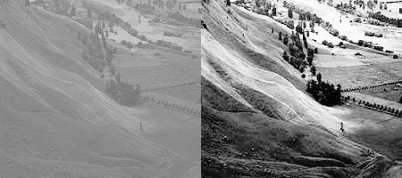
考虑一个图像,其像素值仅限制在特定的值范围内。例如,更明亮的图像将使所有像素都限制在高值中。但是一个好的图像会有来自图像的所有区域的像素。所以你需要把这个直方图拉伸到两端(如下图所给出的),这就是直方图均衡的作用(用简单的话说)。这通常会改善图像的对比度。

建议阅读关于直方图均衡的wikipedia页面Histogram Equalization,了解更多有关它的详细信息。它给出了一个很好的解释,给出了一些例子,这样你就能在读完之后理解所有的东西。同样,我们将看到它的Numpy实现。之后,我们将看到OpenCV函数。
直方图均衡化算法
from 《计算机视觉-算法与应用》 Richard Szeliski
通过亮度和增益的控制可以改善图像的显示,那么我们怎么自动选择它们的最佳取值呢?一种方法是寻找图像中最亮和最暗的像素值,将他们映射到纯白和纯黑。另一种方法是寻找图像中像素值的平均值作为中间灰度值,然后扩展范围以达到尽量充满可显示的值。
对图像进行直方图均衡化,即寻找一个映射函数f(I),经过映射后的直方图是平坦的。寻找此映射的方法与从概率密度分布函数产生随机样本的方法类似,其中首先要计算累计分布函数,
可以把原始的直方图h(I)堪称一个班级在某次考试后的成绩分布。在一个特定的乘积和其学生所占百分比之间,怎样建立映射可以是分数为总分75%以上的学生得分优于班里3/4的同学?答案是通过h(I)的分布得到累计分布函数c(I)
c(I) = \frac{1}{N}\sum_{i=0}^{I}h(i) = c(I-1)+\frac{1}{N}h(I)
- 1
累计分布函数(cumulative distribution function,简称CDF)定义:对于连续函数,所有小于等于a的值,其出现的概率的和。F(a) = P(x<=a)
其中N是图像中像素的总个数或班级中学生的总人数。对于任意给定的成绩或亮度,我们可以查出它对应的百分比c(I),此时可以决定此像素所对应的最终的值。当对8位的像素的值进行操作时,坐标轴I和c要缩放到(0, 255)

其中cdf_min是累积分布函数的最小非零值(在这种情况下为1),M×N给出图像的像素数(对于64以上的例子,其中M是宽度,N是高度),L是使用的灰度级数(在大多数情况下,像这个256一样)。
那么均衡图像的值直接从标准化的cdf中获得以产生均衡值:
Numpy中的直方图均衡化
Numpy相关函数
计算累计和cumsun()
numpy.cumsum(a, axis=None, dtype=None, out=None)
- 1
这个函数的功能是返回给定axis上的累计和
>>>import numpy as np
>>> b=[1,2,3,4,5,6,7]
>>> np.cumsum(a)
array([  1,   3,   6,  10,  15,  21,  28,  36,  45,  55,  75, 105])
- 1
- 2
- 3
- 4
直方图均衡化
import numpy as np
import cv2 as cv
from matplotlib import pyplot as plt

img = cv.imread('wiki.jpg', 0)

hist, bins = np.histogram(img.flatten(), 256, [0,256])

cdf = hist.cumsum()
cdf_normalized = cdf*float(hist.max())/cdf.max()

plt.plot(cdf_normalized, color = 'b')
plt.hist(img.flatten(),256,[0,256], color = 'r')
plt.xlim([0,256])
plt.legend(('cdf','histogram'), loc = 'upper left')
plt.show()
- 1
- 2
- 3
- 4
- 5
- 6
- 7
- 8
- 9
- 10
- 11
- 12
- 13
- 14
- 15
- 16
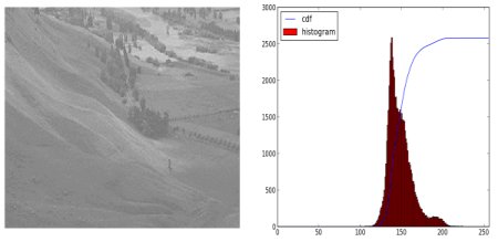
你可以看到直方图位于更亮的区域。我们需要让它充满整个频谱。为此,我们需要一个转换函数,它将更亮区域的输入像素映射到全区域的输出像素。这就是直方图均衡所做的。
现在我们找到了最小的直方图值(不包括0),并应用了在wiki页面中给出的直方图均衡等式。
cdf = (cdf-cdf[0]) *255/ (cdf[-1]-1)
cdf = cdf.astype(np.uint8)
- 1
- 2
现在我们有了一个查找表,它提供了关于每个输入像素值的输出像素值的信息。所以我们只要应用变换。
img2 = cdf[img]
- 1
现在我们计算它的直方图和cdf,就像之前一样,结果如下:
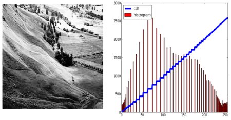
另一个重要的特征是,即使图像是一个较暗的图像(而不是我们使用的更亮的图像),在均衡之后,我们将得到几乎相同的图像。因此,它被用作一种“参考工具”,使所有的图像都具有相同的光照条件。这在很多情况下都很有用。例如,在人脸识别中,在对人脸数据进行训练之前,人脸的图像是均匀的,使它们具有相同的光照条件。
示例1:单通道的灰阶图的直方图均衡化
import cv2 as cv
import numpy as np
from matplotlib import pyplot as plt

img = cv.imread("D:\\CvPic\\test.png", 0)
cv.imshow("before", img)

# calculate hist
hist, bins = np.histogram(img, 256)
# calculate cdf
cdf = hist.cumsum()
# plot hist
plt.plot(hist,'r')

# remap cdf to [0,255]
cdf = (cdf-cdf[0])*255/(cdf[-1]-1)
cdf = cdf.astype(np.uint8)# Transform from float64 back to unit8

# generate img after Histogram Equalization
img2 = np.zeros((384, 495, 1), dtype =np.uint8)
img2 = cdf[img]

hist2, bins2 = np.histogram(img2, 256)
cdf2 = hist2.cumsum()
plt.plot(hist2, 'g')

cv.imshow("after", img2)
plt.show()
cv.waitKey(0)
- 1
- 2
- 3
- 4
- 5
- 6
- 7
- 8
- 9
- 10
- 11
- 12
- 13
- 14
- 15
- 16
- 17
- 18
- 19
- 20
- 21
- 22
- 23
- 24
- 25
- 26
- 27
- 28
- 29
我们可以看到,直方图均衡化后的图像对比度增强了。
示例2:彩图的直方图均衡化
首先是分离通道,对三个通道分别进行处理,合并三通道颜色到图片
import cv2 as cv
import numpy as np
from matplotlib import pyplot as plt


img = cv.imread("D:\\CvPic\\test.png")
cv.imshow("before", img)

# split g,b,r
g = img[:,:,0]
b = img[:,:,1]
r = img[:,:,2]

# calculate hist
hist_r, bins_r = np.histogram(r, 256)
hist_g, bins_g = np.histogram(g, 256)
hist_b, bins_b = np.histogram(b, 256)

# calculate cdf
cdf_r = hist_r.cumsum()
cdf_g = hist_g.cumsum()
cdf_b = hist_b.cumsum()

# remap cdf to [0,255]
cdf_r = (cdf_r-cdf_r[0])*255/(cdf_r[-1]-1)
cdf_r = cdf_r.astype(np.uint8)# Transform from float64 back to unit8
cdf_g = (cdf_g-cdf_g[0])*255/(cdf_g[-1]-1)
cdf_g = cdf_g.astype(np.uint8)# Transform from float64 back to unit8
cdf_b = (cdf_b-cdf_b[0])*255/(cdf_b[-1]-1)
cdf_b = cdf_b.astype(np.uint8)# Transform from float64 back to unit8

# get pixel by cdf table
r2 = cdf_r[r]
g2 = cdf_g[g]
b2 = cdf_b[b]

# merge g,b,r channel
img2 = img.copy()
img2[:,:,0] = g2
img2[:,:,1] = b2
img2[:,:,2] = r2

# show img after histogram equalization
cv.imshow("img2", img2)

cv.waitKey(0)
- 1
- 2
- 3
- 4
- 5
- 6
- 7
- 8
- 9
- 10
- 11
- 12
- 13
- 14
- 15
- 16
- 17
- 18
- 19
- 20
- 21
- 22
- 23
- 24
- 25
- 26
- 27
- 28
- 29
- 30
- 31
- 32
- 33
- 34
- 35
- 36
- 37
- 38
- 39
- 40
- 41
- 42
- 43
- 44
- 45
- 46
示例3:带遮罩的直方图均衡化
如果想要在做直方图均衡化的时候不考虑图像的某一部分,比如我们不想考虑图片右上角的云彩,那么可以使用遮罩在计算hist和cdf时不考虑这一部分像素。
import cv2 as cv
import numpy as np
from matplotlib import pyplot as plt


img = cv.imread("D:\\CvPic\\test.png", 0)
cv.imshow("src", img)

# load mask img
mask = cv.imread("D:\\CvPic\\test_mask2.png", 0)
cv.imshow("mask", mask)

# apply mask to src
masked_img = np.ma.masked_array(img, mask = mask)
masked_img = np.ma.filled(masked_img,0).astype('uint8')
# print(masked_img)
masked_img = np.ma.masked_equal(masked_img,0)
# print(masked_img)
cv.imshow("masked_img", masked_img)


# calculate hist
hist, bins = np.histogram(masked_img.compressed(), 256) # img have to be compressed() to let mask work
# calculate cdf
cdf = hist.cumsum()

print(cdf)
# plot hist
plt.plot(hist,'r')

# remap cdf to [0,255]
cdf = (cdf-cdf[0])*255/(cdf[-1]-1)
cdf = cdf.astype(np.uint8)# Transform from float64 back to unit8

# generate img after Histogram Equalization
img2 = np.zeros((384, 495, 1), dtype =np.uint8)
img2 = cdf[img]

hist2, bins2 = np.histogram(img2, 256)
cdf2 = hist2.cumsum()
plt.plot(hist2, 'g')

cv.imshow("dst", img2)
plt.show()
cv.waitKey(0)
- 1
- 2
- 3
- 4
- 5
- 6
- 7
- 8
- 9
- 10
- 11
- 12
- 13
- 14
- 15
- 16
- 17
- 18
- 19
- 20
- 21
- 22
- 23
- 24
- 25
- 26
- 27
- 28
- 29
- 30
- 31
- 32
- 33
- 34
- 35
- 36
- 37
- 38
- 39
- 40
- 41
- 42
- 43
- 44
- 45
可以看出图片的大楼部分对比度更强烈了。
How to create the histogram of an array with masked values, in Numpy?
OpenCV中的直方图均衡化
OpenCV有一个函数可以这样做,cv.equalizeHist(),它封装好了计算cdf和cdf重映射以及根据cdf表生成直方图均衡图像的过程。它的输入只是灰度图像,输出是我们的直方图均衡图像。
img = cv.imread('wiki,jpg', 0)
equ = cv.equalizeHist(img)
res = np.hstack((img, equ)) # 并排叠加图片
cv.imwrite('res.png', res)
- 1
- 2
- 3
- 4
所以现在你可以用不同的光条件来拍摄不同的图像,平衡它,并检查结果。
当图像的直方图被限制在一个特定的区域时,直方图均衡是很好的。在那些有很大强度变化的地方,直方图覆盖了一个大区域,比如明亮的和暗的像素,这样的地方就不好用了。
示例1:单通道的灰阶图的直方图均衡化
import cv2 as cv
import numpy as np
from matplotlib import pyplot as plt


im = cv.imread("D:\\CvPic\\test.png", 0)
cv.imshow("before", im)

# Histogram Equalization
im2 = cv.equalizeHist(im)
print(im2)

cv.imshow("after", im2)
plt.show()
cv.waitKey(0)
- 1
- 2
- 3
- 4
- 5
- 6
- 7
- 8
- 9
- 10
- 11
- 12
- 13
- 14
- 15
示例2:彩图的直方图均衡
import cv2 as cv
import numpy as np
from matplotlib import pyplot as plt


im = cv.imread("D:\\CvPic\\test.jpg")
cv.imshow("before", im)

# split g,b,r
g = im[:,:,0]
b = im[:,:,1]
r = im[:,:,2]


# Histogram Equalization
r2 = cv.equalizeHist(r)
g2 = cv.equalizeHist(g)
b2 = cv.equalizeHist(b)

im2 = im.copy()
im2[:,:,0] = g2
im2[:,:,1] = b2
im2[:,:,2] = r2

print(im2)

cv.imshow("after", im2)
plt.show()
cv.waitKey(0)
- 1
- 2
- 3
- 4
- 5
- 6
- 7
- 8
- 9
- 10
- 11
- 12
- 13
- 14
- 15
- 16
- 17
- 18
- 19
- 20
- 21
- 22
- 23
- 24
- 25
- 26
- 27
- 28
- 29
示例3:带遮罩的直方图均衡化
import cv2 as cv
import numpy as np
from matplotlib import pyplot as plt

im = cv.imread("D:\\CvPic\\test.png", 0)
cv.imshow("before", im)
mask = cv.imread("D:\\CvPic\\test_mask2.png", 0)
cv.imshow("mask", mask)

# calculate histogram with mask
hist_mask = cv.calcHist([im], [0], mask, [256], [0,256])

# calculate cdf with mask
cdf = hist_mask.cumsum()

# Histogram Equalization
cdf = (cdf-cdf[0])*255/(cdf[-1]-1)
cdf = cdf.astype(np.uint8)# Transform from float64 back to unit8

# generate img after Histogram Equalization
im2 = np.zeros((384, 495, 1), dtype =np.uint8)
im2 = cdf[im]

# im2 = cv.equalizeHist(im)
print(im2)

cv.imshow("after", im2)
plt.show()
cv.waitKey(0)
- 1
- 2
- 3
- 4
- 5
- 6
- 7
- 8
- 9
- 10
- 11
- 12
- 13
- 14
- 15
- 16
- 17
- 18
- 19
- 20
- 21
- 22
- 23
- 24
- 25
- 26
- 27
- 28
- 29
CLAHE(对比有限的自适应直方图均衡/Contrast Limited Adaptive Histogram Equalization)
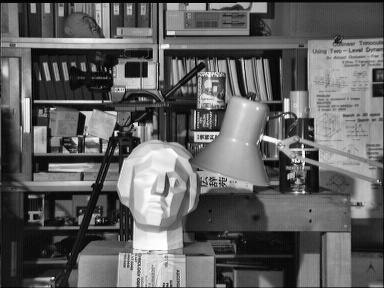
我们刚刚看到的第一个直方图均衡化,考虑到图像的全局对比。在很多情况下,这不是一个好主意。例如,下图显示了一个输入图像及其在全局直方图均衡之后的结果。
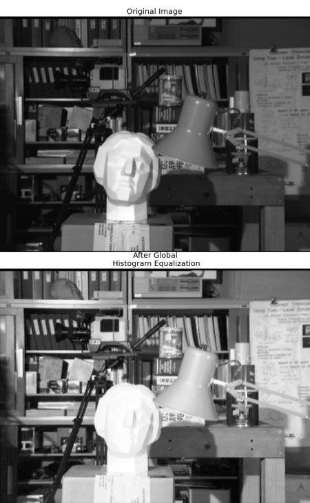
在直方图均衡化之后,背景对比得到了改善。但是比较两幅图像中的雕像的脸。由于亮度过高,我们丢失了大部分的信息。这是因为它的直方图并不局限于一个特定的区域,就像我们在前面的例子中看到的那样。
为了解决这个问题,可以使用了自适应直方图均衡。在这一点上,图像被划分为几个小块,称为“tiles”(在OpenCV中默认值是8x8)。然后每一个方块都是像平常一样的直方图。因此,直方图会限制在一个小区域(除非有噪声)。如果噪音在那里,它就会被放大。为了避免这种情况,会应用对比限制。如果任何直方图bin超出指定的对比度限制(默认情况下是40),在应用直方图均衡之前,这些像素被裁剪并均匀地分布到其他bin。均衡后,删除边界中的工件,采用双线性插值。
cv.createCLAHE([, clipLimit[, tileGridSize]])
- 1
import numpy as np
import cv2 as cv

img = cv.imread('tsukuba_1.png', 0)

# create a CLAHE object (Arguments are optional).
clahe = cv.createCLAHE(clipLimit=2.0, tileGridSize=(8,8))
cl1 = clahe.apply(img)

cv.imread('clahe_2.jpg', cl1)
- 1
- 2
- 3
- 4
- 5
- 6
- 7
- 8
- 9
- 10