【python】PIL（下）

版权声明：本文为博主原创文章，未经博主允许不得转载。 https://blog.csdn.net/bryant_meng/article/details/86185490

参考：

• 【python】matplotlib
• Python计算机视觉3：模糊,平滑,去噪

上一篇：

• 【python】PIL（上）

转载+整理+扩充：

• python计算机视觉2：图像边缘检测
• 【计算机视觉】卷积、均值滤波、高斯滤波、Sobel算子、Prewitt算子(Python实现)

---

---

PIL 模块全称为 Python Imaging Library，是python中一个免费的图像处理模块。

1 导数，梯度，边缘信息

在数学中，与变化率有关的就是导数。
如果灰度图像的像素是连续的(实际不是)，那么我们可以分别原图像 $G$ 对 $x$ 方向和 $y$ 方向求导数 $G_x = \frac{\partial G}{\partial x}$， $G_y = \frac{\partial G}{\partial y}$
获得 $x$ 方向的导数图像 $G_x$ 和 $y$ 方向的导数图像 $G_y$。 $G_x$ 和 $G_y$ 分别隐含了 $x$ 和 $y$ 方向的灰度变化信息，也就隐含了边缘信息。如果要在同一图像上包含两个方向的边缘信息，我们可以用到梯度。（梯度是一个向量）
原图像的梯度向量 $G_{xy}$为（ $G_x$, $G_y$）,梯度向量的大小和方向可以用下面两个式子计算
$\left | G_{xy} \right |=\sqrt{G_{x}^{2} + G_{y}^{2}}$， $\angle G_{xy} = arctan\left ( \frac{G_{y}}{G_{x}} \right )$

• 角度值好像需要根据向量所在象限不同适当 + $\pi$ 或者 - $\pi$。
• 梯度向量大小就包含了 $x$ 方向和 $y$ 方向的边缘信息。

2 图像导数

实际上，图像矩阵是离散的。连续函数求变化率用的是导数，而离散函数求变化率用的是差分。差分的概念很容易理解，就是用相邻两个数的差来表示变化率。
实际计算图像导数时，我们是通过原图像和一个算子进行卷积来完成的（这种方法是求图像的近似导数）。最简单的求图像导数的算子是 Prewitt 算子 ：
$x$ 方向的 Prewitt 算子为： $\begin{bmatrix} -1 & 0& 1\\ -1 & 0& 1\\ -1 & 0& 1 \end{bmatrix}$

$y$ 方向的 Prewitt 算子为： $\begin{bmatrix} -1 & -1& -1\\ 0 & 0& 0\\ 1 & 1& 1 \end{bmatrix}$

卷积过程如下（准确来说是相关，don’t care），虚线表示 padding 部分，下面蓝色的是原图，上面绿色的是卷积以后的图，下面滑动的9宫格就是我们定义的 $x$ 方向的 Prewitt 算子、 $y$ 方向的 Prewitt 算子

因此，利用原图像和 $x$ 方向 Prewitt 算子进行卷积就可以得到图像的 $x$ 方向导数矩阵 $G_x$，利用原图像和 $y$ 方向 Prewitt 算子进行卷积就可以得到图像的 $y$ 方向导数矩阵 $G_y$。

利用公式 $\left | G_{xy} \right |=\sqrt{G_{x}^{2} + G_{y}^{2}}$，就可以得到图像的梯度矩阵 $G_{xy}$，这个矩阵包含图像 $x$ 方向和 $y$ 方向的边缘信息。

3 Prewitt 算子的边缘检测

实际上，scipy库中的signal模块含有一个二维卷积的方法 convolve2d() ，造轮子可以参考博客【计算机视觉】卷积、均值滤波、高斯滤波、Sobel算子、Prewitt算子(Python实现)

3.1 造轮子

1）定义卷积

import numpy as np
from PIL import Image
import matplotlib.pyplot as plt
# 卷积
def imgConvolve(image, kernel):
    '''
    :param image: 图片矩阵
    :param kernel: 滤波窗口
    :return:卷积后的矩阵
    '''
    img_h = int(image.shape[0])
    img_w = int(image.shape[1])
    kernel_h = int(kernel.shape[0])
    kernel_w = int(kernel.shape[1])
    # padding
    padding_h = int((kernel_h - 1) / 2)
    padding_w = int((kernel_w - 1) / 2)

    convolve_h = int(img_h + 2 * padding_h)
    convolve_W = int(img_w + 2 * padding_w)

    # 分配空间
    img_padding = np.zeros((convolve_h, convolve_W))
    # 中心填充图片
    img_padding[padding_h:padding_h + img_h, padding_w:padding_w + img_w] = image[:, :]
    # 卷积结果
    image_convolve = np.zeros(image.shape)
    # 卷积
    for i in range(padding_h, padding_h + img_h):
        for j in range(padding_w, padding_w + img_w):
            image_convolve[i - padding_h][j - padding_w] = int(
                np.sum(img_padding[i - padding_h:i + padding_h+1, j - padding_w:j + padding_w+1]*kernel))

    return image_convolve

2）定义算子

# x方向的Prewitt算子
operator_x = np.array([[-1, 0, 1],
                       [ -1, 0, 1],
                       [ -1, 0, 1]])
# y方向的Prewitt算子
operator_y = np.array([[-1,-1,-1],
                       [ 0, 0, 0],
                       [ 1, 1, 1]])

3）计算并可视化结果

image = Image.open("C://Users/13663//Desktop/1.jpg").convert("L")
image_array = np.array(image)
image_x = imgConvolve(image_array,operator_x)
image_y = imgConvolve(image_array,operator_y)
image_xy = np.sqrt(image_x**2+image_y**2)
# 绘出图像，灰度图
plt.subplot(2,2,1)
plt.imshow(image_array,cmap='gray')
plt.title('the grey-scale image',size=15,color='w')
plt.axis("off")
# x 方向的梯度
plt.subplot(2,2,2)
plt.imshow(image_x,cmap='gray')
plt.title('the derivative of x',size=15,color='w')
plt.axis("off")
# y 方向导数图像
plt.subplot(2,2,3)
plt.imshow(image_y,cmap='gray')
plt.title('the derivative of y',size=15,color='w')
plt.axis("off")
# 梯度图像
plt.subplot(2,2,4)
plt.imshow(image_xy,cmap='gray')
plt.title('the gradient of image',size=15,color='w')
plt.axis("off")
plt.show()

3.2 它山之石可以攻玉

调用 scipy 中的 signal.convolve2d

import numpy as np
from PIL import Image
import matplotlib.pyplot as plt
import scipy.signal as signal     # 导入sicpy的signal模块
# x方向的Prewitt算子
operator_x = np.array([[-1, 0, 1],
                       [ -1, 0, 1],
                       [ -1, 0, 1]])
# y方向的Prewitt算子
operator_y = np.array([[-1,-1,-1],
                       [ 0, 0, 0],
                       [ 1, 1, 1]])

# 打开图像并转化成灰度图像
image = Image.open("C://Users/13663//Desktop/2.jpg").convert("L")
image_array = np.array(image)
# 利用signal的convolve计算卷积
image_x = signal.convolve2d(image,operator_x,mode="same")
image_y = signal.convolve2d(image,operator_y,mode="same")
image_xy = np.sqrt(image_x**2+image_y**2)
# 绘出图像，灰度图
plt.subplot(2,2,1)
plt.imshow(image_array,cmap='gray')
plt.title('the grey-scale image',size=15,color='w')
plt.axis("off")
# x 方向的梯度
plt.subplot(2,2,2)
plt.imshow(image_x,cmap='gray')
plt.title('the derivative of x',size=15,color='w')
plt.axis("off")
# y 方向导数图像
plt.subplot(2,2,3)
plt.imshow(image_y,cmap='gray')
plt.title('the derivative of y',size=15,color='w')
plt.axis("off")
# 梯度图像
plt.subplot(2,2,4)
plt.imshow(image_xy,cmap='gray')
plt.title('the gradient of image',size=15,color='w')
plt.axis("off")
plt.show()

对比下造轮子和调用的结果

左边是造轮子的结果，右边是调用的结果，会注意到 the derivative of x 和 the derivative of y 中略有差异，粗略的看造轮子中是黑线（0），而调用中是白线（255），仔细对比发现，他们各个位置的像素值好像是互补的（相加=255），输出卷积后数组最大值和最小值会发现

print(image_x.max())
print(image_x.min())

造轮子的 output 为

411.0
-477.0

调用的 output 为

477
-411

哈哈哈，确实是正好反过来了，matplotlib 画图时会归一化到0-255，所以两者在可视化中互补为255，nice
修改造轮子代码中 def imgConvolve(image, kernel): 函数的输出为原来的相反数 return -image_convolve，再试试

左边为造轮子代码，右边为调用的代码，ok，一样了

4 Sobel 算子的边缘检测

修改下 operator 即可

# x方向的Sobel算子
operator_x = np.array([[-1, 0, 1],
                       [ -2, 0, 2],
                       [ -1, 0, 1]])
# y方向的Sobel算子
operator_y = np.array([[-1,-2,-1],
                       [ 0, 0, 0],
                       [ 1, 2, 1]])

5 Laplace 算子

Laplace 算子是一个二阶导数的算子，它实际上是一个 $x$ 方向二阶导数和 $y$ 方向二阶导数的和的近似求导算子。实际上，Laplace算子是通过Sobel算子推导出来的。
Laplace算子为 $\begin{bmatrix} 0 & 1& 0\\ 1 & -4& 1\\ 0 & 1& 0 \end{bmatrix}$

Laplace还有一种扩展算子为 $\begin{bmatrix} 1 & 1& 1\\ 1 & -8& 1\\ 1 & 1& 1 \end{bmatrix}$

import numpy as np
from PIL import Image
import matplotlib.pyplot as plt
import scipy.signal as signal     # 导入sicpy的signal模块

# Laplace算子
Laplace1 = np.array([[0, 1, 0],  
                    [1,-4, 1],
                    [0, 1, 0]])

# Laplace扩展算子
Laplace2 = np.array([[1, 1, 1],
                    [1,-8, 1],
                    [1, 1, 1]])

# 打开图像并转化成灰度图像
image = Image.open("C://Users/13663//Desktop/2.jpg").convert("L")
image_array = np.array(image)

# 利用signal的convolve计算卷积
image_1 = signal.convolve2d(image,Laplace1,mode="same")
image_2 = signal.convolve2d(image,Laplace2,mode="same")

可视化结果

laplace 1

plt.imshow(image_1,cmap='gray')
plt.title('laplace 1',size=15,color='w')
plt.axis("off")
plt.show()

laplace 2

plt.imshow(image_2,cmap='gray')
plt.title('laplace 2',size=15,color='w')
plt.axis("off")
plt.show()

视觉效果不是很好，我们加点内容

# 将卷积结果转化成0~255
image_1 = (image_1/float(image_1.max()))*255
image_2 = (image_2/float(image_2.max()))*255

# 为了使看清边缘检测结果，将大于灰度平均值的灰度变成255(白色)
image_1[image_1>image_1.mean()] = 255
image_2[image_2>image_2.mean()] = 255

看另外一个例子


改进视觉效果

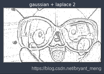
6 Gaussian + Laplace

先来个 Gaussian 模糊，然后再 滤波
$G\left ( x,y \right )=\frac{1}{2\pi \sigma }e^{\frac{-\left ( x^{2}+y^{2} \right )}{2\sigma^{2} }}$

import numpy as np
from PIL import Image
import matplotlib.pyplot as plt
import scipy.signal as signal

# 乘以100是为了使算子中的数便于观察
# sigma指定高斯算子的标准差

# 生成高斯算子的函数
def func(x,y,sigma=1):
    return 100*(1/(2*np.pi*sigma))*np.exp(-((x-2)**2+(y-2)**2)/(2.0*sigma**2))

# 生成标准差为5的5*5高斯算子
gaussian = np.fromfunction(func,(5,5),sigma=5)

# Laplace扩展算子
laplace2 = np.array([[1, 1, 1],
                     [1,-8, 1],
                     [1, 1, 1]])

# 打开图像并转化成灰度图像
image = Image.open("C://Users/13663//Desktop/1.jpg").convert("L")
image_array = np.array(image)

# 利用生成的高斯算子与原图像进行卷积对图像进行平滑处理
image_blur = signal.convolve2d(image_array, gaussian, mode="same")

# 对平滑后的图像进行边缘检测
image2 = signal.convolve2d(image_blur, laplace2, mode="same")

# 显示图像
plt.imshow(image2,cmap='gray')
plt.axis("off")
plt.title('gaussian + laplace 2',size=15,color='w')
plt.show()

增进下视觉效果，在 image2 = signal.convolve2d(image_blur, laplace2, mode="same") 后加入以下代码

# 结果转化到0-255
image2 = (image2/float(image2.max()))*255

# 将大于灰度平均值的灰度值变成255（白色），便于观察边缘
image2[image2>image2.mean()] = 255

再改下 gaussian = np.fromfunction(func,(3,3),sigma=3)

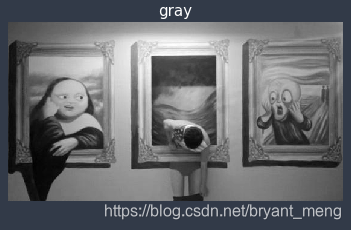
换个图片看看效果



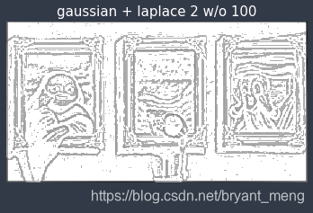
gaussian + laplace 2 w/o 100 表示计算高斯核的时候，没有乘以 100