动态时间规整算法,
就是把两个代表同一个类型的事物的不同长度序列进行时间上的“对齐”。比如DTW最常用的地方,语音识别中,同一个字母,由不同人发音,长短肯定不一样,把声音记录下来以后,它的信号肯定是很相似的,只是在时间上不太对整齐而已。所以我们需要用一个函数拉长或者缩短其中一个信号,使得它们之间的误差达到最小。
在时间序列中,需要比较相似性的两段时间序列的长度可能并不相等,在语音识别领域表现为不同人的语速不同。而且同一个单词内的不同音素的发音速度也不同,比如有的人会把“A”这个音拖得很长,或者把“i”发的很短。另外,不同时间序列可能仅仅存在时间轴上的位移,亦即在还原位移的情况下,两个时间序列是一致的。在这些复杂情况下,使用传统的欧几里得距离无法有效地求的两个时间序列之间的距离(或者相似性)。
DTW通过把时间序列进行延伸和缩短,来计算两个时间序列性之间的相似性:

如上图所示,上下两条实线代表两个时间序列,时间序列之间的虚线代表两个时间序列之间的相似的点。DTW使用所有这些相似点之间的距离的和,称之为归整路径距离(Warp Path Distance)来衡量两个时间序列之间的相似性。
再来看看运动捕捉,比如当前有一个很快的拳击动作,另外有一个未加标签的动作,我想判断它是不是拳击动作,那么就要计算这个未加标签的动作和已知的拳击动作的相似度。但是呢,他们两个的动作长度不一样,比如一个是100帧,一个是200帧,那么这样直接对每一帧进行对比,计算到后面,误差肯定很大,那么我们把已知拳击动作的每一帧找到无标签的动作的对应帧中,使得它们的距离最短。这样便可以计算出两个运动的相似度,然后设定一个阈值,满足阈值范围就把未知动作加上“拳击”标签。
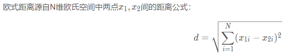
欧式距离的计算方法:

图来自维基百科,其中红黄蓝线均为曼哈顿距离,绿色为欧式距离
DTW的具体计算过程:
下面我们来总结一下DTW动态时间规整算法的简单的步骤:
1. 首先肯定是已知两个或者多个序列,但是都是两个两个的比较,所以我们假设有两个序列A={a1,a2,a3,...,am} B={b1,b2,b3,....,bn},维度m>n
2. 然后用欧式距离计算出每序列的每两点之间的距离,D(ai,bj) 其中1≤i≤m,1≤j≤n
画出下表: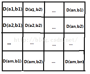
3. 接下来就是根据上图将最短路径找出来。从D(a1,a2)沿着某条路径到达D(am,bn)。找路径满足:假如当前节点是D(ai,bj),那么下一个节点必须是在D(i+1,j),D(i,j+1),D(i+1,j+1)之间选择,并且路径必须是最短的。计算的时候是按照动态规划的思想计算,也就是说在计算到达第(i,j)个节点的最短路径时候,考虑的是左上角也即第(i-1,j)、(i-1,j-1)、(i,j-1)这三个点到(i,j)的最短距离。
4. 接下来按照回溯法输出路径,从D(a1,b1)到D(am,bn)。他们的总和就是就是所需要的DTW距离
举个栗子:
已知:两个列向量a=[8 9 1]',b=[ 2 5 4 6]',其中'代表转置,也就是把行向量转换为列向量了
求:两个向量利用动态时间规整以后的最短距离
第一步:计算对应点的欧式距离矩阵d【注意开根号】
| 6 | 3 | 4 | 2 |
| 7 | 4 | 5 | 3 |
| 1 | 4 | 3 | 5 |
第二步:计算累加距离D【从6出发到达5的累加距离】
| 6 | 9 | 13 | 15 |
| 13 | 10 | 14 | 16 |
| 14 | 14 | 13 | 18 |
计算方法如下:
D(1,1)=d(1,1)=6
D(1,2)=D(1,1)+d(1,2)=9
...
D(2,2)=min(D(1,2),D(1,1),D(2,1))+d(2,2)=6+4=10
...
D(m,n)=min(D(m-1,n),D(m-1,n-1),D(m,n-1))+d(m,n)
matlab的代码如下:
dtw.m
function [Dist,D,k,w,rw,tw]=dtw(r,t,pflag)
%
% [Dist,D,k,w,rw,tw]=dtw(r,t,pflag)
%
% Dynamic Time Warping Algorithm
% Dist is unnormalized distance between t and r
% D is the accumulated distance matrix
% k is the normalizing factor
% w is the optimal path
% t is the vector you are testing against
% r is the vector you are testing
% rw is the warped r vector
% tw is the warped t vector
% pflag plot flag: 1 (yes), 0(no)
%
% Version comments:
% rw, tw and pflag added by Pau Mic
[row,M]=size(r); if (row > M) M=row; r=r'; end;
[row,N]=size(t); if (row > N) N=row; t=t'; end;
d=sqrt((repmat(r',1,N)-repmat(t,M,1)).^2); %this makes clear the above instruction Thanks Pau Mic
d
D=zeros(size(d));
D(1,1)=d(1,1);
for m=2:M
D(m,1)=d(m,1)+D(m-1,1);
end
for n=2:N
D(1,n)=d(1,n)+D(1,n-1);
end
for m=2:M
for n=2:N
D(m,n)=d(m,n)+min(D(m-1,n),min(D(m-1,n-1),D(m,n-1))); % this double MIn construction improves in 10-fold the Speed-up. Thanks Sven Mensing
end
end
Dist=D(M,N);
n=N;
m=M;
k=1;
w=[M N];
while ((n+m)~=2)
if (n-1)==0
m=m-1;
elseif (m-1)==0
n=n-1;
else
[values,number]=min([D(m-1,n),D(m,n-1),D(m-1,n-1)]);
switch number
case 1
m=m-1;
case 2
n=n-1;
case 3
m=m-1;
n=n-1;
end
end
k=k+1;
w=[m n; w]; % this replace the above sentence. Thanks Pau Mic
end
% warped waves
rw=r(w(:,1));
tw=t(w(:,2));
%%%%%%%%%%%%%%%%%%%%%%%%%%%%%%%%%%%%%%%%%%%%%%%%%%%%%%%%%%%%%%%%%%%%%%%%%%%
if pflag
% --- Accumulated distance matrix and optimal path
figure('Name','DTW - Accumulated distance matrix and optimal path', 'NumberTitle','off');
main1=subplot('position',[0.19 0.19 0.67 0.79]);
image(D);
cmap = contrast(D);
colormap(cmap); % 'copper' 'bone', 'gray' imagesc(D);
hold on;
x=w(:,1); y=w(:,2);
ind=find(x==1); x(ind)=1+0.2;
ind=find(x==M); x(ind)=M-0.2;
ind=find(y==1); y(ind)=1+0.2;
ind=find(y==N); y(ind)=N-0.2;
plot(y,x,'-w', 'LineWidth',1);
hold off;
axis([1 N 1 M]);
set(main1, 'FontSize',7, 'XTickLabel','', 'YTickLabel','');
colorb1=subplot('position',[0.88 0.19 0.05 0.79]);
nticks=8;
ticks=floor(1:(size(cmap,1)-1)/(nticks-1):size(cmap,1));
mx=max(max(D));
mn=min(min(D));
ticklabels=floor(mn:(mx-mn)/(nticks-1):mx);
colorbar(colorb1);
set(colorb1, 'FontSize',7, 'YTick',ticks, 'YTickLabel',ticklabels);
set(get(colorb1,'YLabel'), 'String','Distance', 'Rotation',-90, 'FontSize',7, 'VerticalAlignment','bottom');
left1=subplot('position',[0.07 0.19 0.10 0.79]);
plot(r,M:-1:1,'-b');
set(left1, 'YTick',mod(M,10):10:M, 'YTickLabel',10*rem(M,10):-10:0)
axis([min(r) 1.1*max(r) 1 M]);
set(left1, 'FontSize',7);
set(get(left1,'YLabel'), 'String','Samples', 'FontSize',7, 'Rotation',-90, 'VerticalAlignment','cap');
set(get(left1,'XLabel'), 'String','Amp', 'FontSize',6, 'VerticalAlignment','cap');
bottom1=subplot('position',[0.19 0.07 0.67 0.10]);
plot(t,'-r');
axis([1 N min(t) 1.1*max(t)]);
set(bottom1, 'FontSize',7, 'YAxisLocation','right');
set(get(bottom1,'XLabel'), 'String','Samples', 'FontSize',7, 'VerticalAlignment','middle');
set(get(bottom1,'YLabel'), 'String','Amp', 'Rotation',-90, 'FontSize',6, 'VerticalAlignment','bottom');
% --- Warped signals
figure('Name','DTW - warped signals', 'NumberTitle','off');
subplot(1,2,1);
set(gca, 'FontSize',7);
hold on;
plot(r,'-bx');
plot(t,':r.');
hold off;
axis([1 max(M,N) min(min(r),min(t)) 1.1*max(max(r),max(t))]);
grid;
legend('signal 1','signal 2');
title('Original signals');
xlabel('Samples');
ylabel('Amplitude');
subplot(1,2,2);
set(gca, 'FontSize',7);
hold on;
plot(rw,'-bx');
plot(tw,':r.');
hold off;
axis([1 k min(min([rw; tw])) 1.1*max(max([rw; tw]))]);
grid;
legend('signal 1','signal 2');
title('Warped signals');
xlabel('Samples');
ylabel('Amplitude');
end
下面是测试代码
test.m
clear
clc
a=[8 9 1 9 6 1 3 5]';
b=[2 5 4 6 7 8 3 7 7 2]';
[Dist,D,k,w,rw,tw] = DTW(a,b,1);
fprintf('最短距离为%d\n',Dist)
fprintf('最优路径为')
w
测试结果:
d =
6 3 4 2 1 0 5 1 1 6
7 4 5 3 2 1 6 2 2 7
1 4 3 5 6 7 2 6 6 1
7 4 5 3 2 1 6 2 2 7
4 1 2 0 1 2 3 1 1 4
1 4 3 5 6 7 2 6 6 1
1 2 1 3 4 5 0 4 4 1
3 0 1 1 2 3 2 2 2 3
最短距离为27
最优路径为
w =
1 1
1 2
1 3
1 4
1 5
1 6
2 6
3 7
4 8
5 9
6 10
7 10
8 10
规整以后的可视化结果如下:


---------------------
作者:风翼冰舟
来源:CSDN
原文:https://blog.csdn.net/zb1165048017/article/details/49226315
版权声明:本文为博主原创文章,转载请附上博文链接!