Python实现前向逐步回归

当基于最小二乘法训练线性回归模型而发生过拟合现象时，最小二乘法没有办法阻止学习过程。前向逐步回归的引入则可以控制学习过程中出现的过拟合，它是最小二乘法的一种改进或者说调整，其基本思想是由少到多地向模型中引入变量，每次增加一个，直到没有可以引入的变量为止。最后通过比较在预留样本上计算出的错误进行模型的选择。

实现代码如下：

# 导入要用到的各种包和函数
import numpy as np
import pandas as pd
from sklearn import datasets, linear_model
from math import sqrt
import matplotlib.pyplot as plt

# 读入要用到的红酒数据集
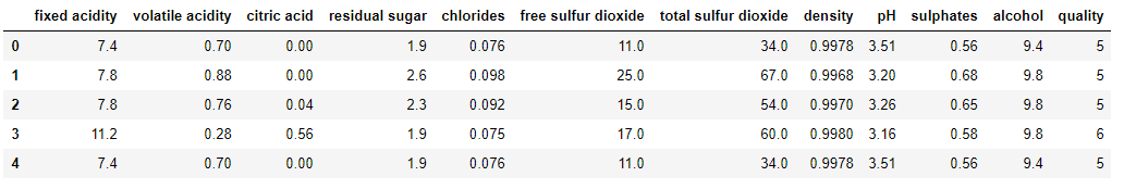
wine_data = pd.read_csv('wine.csv')
wine_data.head()

wine_data的表结构如下图所示：

# 查看红酒数据集的统计信息
wine_data.describe()

wine_data中部分属性的统计信息如下：

# 定义从输入数据集中取指定列作为训练集和测试集的函数(从取1列一直到取11列):
def xattrSelect(x, idxSet):
    xOut = []
    for row in x:
        xOut.append([row[i] for i in idxSet])
    return(xOut)


xList = []  # 构造用于存放属性集的列表
labels = [float(label) for label in wine_data.iloc[:,-1].tolist()]  # 提取出wine_data中的标签集并放入列表中
names = wine_data.columns.tolist()          # 提取出wine_data中所有属性的名称并放入列表中
for i in range(len(wine_data)):
    xList.append(wine_data.iloc[i,0:-1])    # 列表xList中的每个元素对应着wine_data中除去标签列的每一行

# 将原始数据集划分成训练集(占2/3)和测试集(占1/3)：
indices = range(len(xList))
xListTest = [xList[i] for i in indices if i%3 == 0 ]
xListTrain = [xList[i] for i in indices if i%3 != 0 ]
labelsTest = [labels[i] for i in indices if i%3 == 0]
labelsTrain = [labels[i] for i in indices if i%3 != 0]


attributeList = []            # 构造用于存放属性索引的列表
index = range(len(xList[1]))  # index用于下面代码中的外层for循环
indexSet = set(index)         # 构造由names中的所有属性对应的索引构成的索引集合
oosError = []                 # 构造用于存放下面代码中的内层for循环每次结束后最小的RMSE


for i in index:
    attSet = set(attributeList)
    attTrySet = indexSet - attSet          # 构造由不在attributeList中的属性索引组成的集合
    attTry = [ii for ii in attTrySet]      # 构造由在attTrySet中的属性索引组成的列表
    errorList = []
    attTemp = []
    
    for iTry in attTry:
        attTemp = [] + attributeList
        attTemp.append(iTry)
        
        # 调用attrSelect函数从xListTrain和xListTest中选取指定的列构成暂时的训练集与测试集
        xTrainTemp = xattrSelect(xListTrain, attTemp)
        xTestTemp = xattrSelect(xListTest, attTemp)
        
        # 将需要用到的训练集和测试集都转化成数组对象
        xTrain = np.array(xTrainTemp) 
        yTrain = np.array(labelsTrain)
        xTest = np.array(xTestTemp)
        yTest = np.array(labelsTest)
        
        # 使用scikit包训练线性回归模型
        wineQModel = linear_model.LinearRegression()
        wineQModel.fit(xTrain,yTrain)
        
        # 计算在测试集上的RMSE
        rmsError = np.linalg.norm((yTest-wineQModel.predict(xTest)), 2)/sqrt(len(yTest)) # 利用向量的2范数计算RMSE
        errorList.append(rmsError)
        attTemp = []
        
    iBest = np.argmin(errorList)          # 选出errorList中的最小值对应的新索引
    attributeList.append(attTry[iBest])   # 利用新索引iBest将attTry中对应的属性索引添加到attributeList中
    oosError.append(errorList[iBest])     # 将errorList中的最小值添加到oosError列表中

print("Out of sample error versus attribute set size" )
print(oosError)
print("\n" + "Best attribute indices")
print(attributeList)
namesList = [names[i] for i in attributeList]
print("\n" + "Best attribute names")
print(namesList)

上述代码的输出结果为：

Out of sample error versus attribute set size
[0.7234259255146811, 0.6860993152860264, 0.6734365033445415, 0.6677033213922949, 
0.6622558568543597, 0.6590004754171893, 0.6572717206161052, 0.6570905806225685, 
0.6569993096464123, 0.6575818940063175, 0.6573909869028242]

Best attribute indices
[10, 1, 9, 4, 6, 8, 5, 3, 2, 7, 0]

Best attribute names
['alcohol', 'volatile acidity', 'sulphates', 'chlorides', 'total sulfur dioxide', 'pH', 
'free sulfur dioxide', 'residual sugar', 'citric acid', 'density', 'fixed acidity']

# 绘制由不同数量的属性构成的线性回归模型在测试集上的RMSE与属性数量的关系图像
x = range(len(oosError))
plt.plot(x, oosError, 'k')
plt.xlabel('Number of Attributes')
plt.ylabel('Error (RMS)')
plt.show()

# 绘制由最佳数量的属性构成的线性回归模型在测试集上的误差分布直方图
indexBest = oosError.index(min(oosError))
attributesBest = attributeList[1:(indexBest+1)]   # attributesBest包含8个属性索引

# 调用xattrSelect函数从xListTrain和xListTest中选取最佳数量的列组成暂时的训练集和测试集
xTrainTemp = xattrSelect(xListTrain, attributesBest)
xTestTemp = xattrSelect(xListTest, attributesBest)
xTrain = np.array(xTrainTemp)    # 将xTrain转化成数组对象
xTest = np.array(xTestTemp)      # 将xTest转化成数组对象

# 训练模型并绘制直方图
wineQModel = linear_model.LinearRegression()
wineQModel.fit(xTrain,yTrain)
errorVector = yTest-wineQModel.predict(xTest)
plt.hist(errorVector)
plt.xlabel("Bin Boundaries")
plt.ylabel("Counts")
plt.show()

# 绘制红酒口感实际值与预测值之间的散点图
plt.scatter(wineQModel.predict(xTest), yTest, s=100, alpha=0.10)
plt.xlabel('Predicted Taste Score')
plt.ylabel('Actual Taste Score')
plt.show()

上述代码绘制的图像如下：

RMSE与属性数量的关系图像：

错误直方图：

实际值与预测值的散点图：

参考：

《Python机器学习——预测分析核心算法》Michael Bowles著

https://baike.baidu.com/item/%E9%80%90%E6%AD%A5%E5%9B%9E%E5%BD%92/585832?fr=aladdin

https://blog.csdn.net/qq_41080850/article/details/86506408

Python实现前向逐步回归

猜你喜欢