My First SLAM Implementation EKF-SLAM

版权声明：本文为博主原创文章，未经博主允许不得转载，否则将通知维权骑士维护自己的权益。 https://blog.csdn.net/c602273091/article/details/52695612

转载请注明出处：http://blog.csdn.net/c602273091/article/details/52695612

ABSTRACT

Learn by doing !

To do it with EKF-SLAM, you can have better comprehensive understanding of SLAM.

---

PRINCIPLE

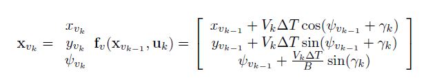
State update by control：（here the control is applied with noise）

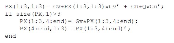
Calculate Predict Covariance:

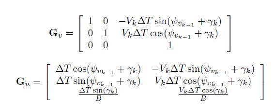
The Jacobian $Gv$ and $Gu$ are calculated by:

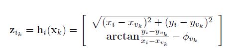
The sensor model is update by:

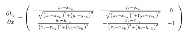
And the Jacobian for robot state is:

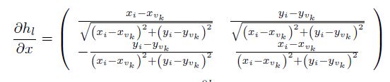
the Jacobian for land mark is:

For more details for EKF, search WiKi with EKF.

---

IMPLEMENTATION

% function my_efk_slam
function my_ekf_2d_slam
    %% load data
    format compact;
    load('example_webmap'); % store in lm, wp
    fig = figure;
    plot(lm(1,:), lm(2,:), 'b*');
    hold on;
    axis equal;
    plot(wp(1,:), wp(2,:), 'g', wp(1,:), wp(2,:), 'g.');
    xlabel('meters'), ylabel('meters');
    set(fig, 'name', 'My 2D EKF-SLAM');

    %% load parameter
    V = 3;% m/s
    MAXG  = 30*pi/180.0;  % maximum steering angles
    RATEG = 20*pi/180.0; % maximum rate of change steering angles
    WHEELBASE   = 4;    % vihecle base
    DT_CONTROLS = 0.025; % seconds between control signals
    sigmaV = 0.3;       % m/s
    sigmaG = (3.0*pi/180); %radians
    Q      = [sigmaV^2 0; 0 sigmaG^2];
    MAX_RANGE = 30.0;   % meters.
    DT_OBSERVE = 8*DT_CONTROLS; % time between observation
    sigmaR = 0.1; 
    sigmaB = (1.0*pi/180);
    R = [sigmaR^2 0; 0 sigmaB^2];
    GATE_REJECT = 4.0;  % maximum dis for creation of new feature.
    GATE_AUGMENT = 25.0; % minimum dis for creation new feature.
    AT_WAYPOINT = 1.0;
    NUMBER_LOOPS = 2; % number of loops through the waypoint list.
    SWITCH_CONTROL_NOISE= 1; % if 0, velocity and gamma are perfect
    SWITCH_SENSOR_NOISE = 1; % if 0, measurements are perfect
    SWITCH_INFLATE_NOISE= 0; % if 1, the estimated Q and R are inflated (ie, add stabilising noise)
    SWITCH_HEADING_KNOWN= 0; % if 1, the vehicle heading is observed directly at each iteration
    SWITCH_ASSOCIATION_KNOWN= 0; % if 1, associations are given, if 0, they are estimated using gates
    SWITCH_BATCH_UPDATE= 1; % if 1, process scan in batch, if 0, process sequentially
    SWITCH_SEED_RANDOM= 0; % if not 0, seed the randn() with its value at beginning of simulation (for repeatability)
    SWITCH_USE_IEKF= 0; % if 1, use iterated EKF for updates, if 0, use normal EKF
    if SWITCH_INFLATE_NOISE, QE= 2*Q; RE= 8*R; end % inflate estimated noises (ie, add stabilising noise)
    if SWITCH_SEED_RANDOM, randn('state',SWITCH_SEED_RANDOM), end
    %% set up animations
    h.xt = patch(0, 0, 'b', 'erasemode', 'xor');
    h.xv = patch(0, 0, 'r', 'erasemode', 'xor'); % vehicle
    h.pth= plot(0,0,'k.','markersize',2,'erasemode','background'); % vehicle path estimate
    h.obs= plot(0,0,'r','erasemode','xor'); % observations
    h.xf = plot(0,0,'r+','erasemode','xor'); % estimated features
    h.cov= plot(0,0,'r','erasemode','xor'); % covariance ellipses
    veh  = [0 -WHEELBASE -WHEELBASE;0 -2 2];
    pcount  = 0;

    %% initialization
    xtrue = zeros(3, 1);
    x = zeros(3, 1);
    P = zeros(3);
    dt = DT_CONTROLS;
    dtsum = 0;
    ftag = 1:size(lm,2);
    da_table = zeros(1,size(lm,2));
    iwp = 1;
    G = 0;

    %% stored data for off-line
    data.i = 1;
    data.path = x;
    data.true = xtrue;
    data.state(1).x = x;
    data.state(1).P = diag(P);

    QE = Q;
    RE = R;

    % main loop 
    while iwp ~= 0
        %% compute steering [G,iwp]= compute_steering(xtrue, wp, iwp, AT_WAYPOINT, G, RATEG, MAXG, dt);
         cwp = wp(:, iwp);
         d2 = (cwp(1) - xtrue(1))^2 + (cwp(2) - xtrue(2))^2;
         if d2 < AT_WAYPOINT^2
             iwp = iwp + 1;
             if iwp > size(wp, 2)
                 iwp = 0;
             end   
             if iwp ~= 0
                cwp = wp(:, iwp);
             end   
         end
         if iwp ~= 0
            deltaG = pi_to_pi(atan2(cwp(2) - xtrue(2), cwp(1) - xtrue(1)) - xtrue(3) - G);
             maxDelta = RATEG*dt;

            if abs(deltaG) > maxDelta
                 deltaG = sign(deltaG)*maxDelta;
            end    
            G = G + deltaG;
            if abs(G) > MAXG
                 G = sign(G)*MAXG;
            end
         end

         %[G,iwp]= compute_steering(xtrue, wp, iwp, AT_WAYPOINT, G, RATEG, MAXG, dt);
         if iwp == 0 && NUMBER_LOOPS > 1, iwp = 1; NUMBER_LOOPS = NUMBER_LOOPS - 1;  disp(NUMBER_LOOPS); end;

        %% xtrue= vehicle_model(xtrue, V,G, WHEELBASE,dt);
         xtrue = [xtrue(1) + V * dt * cos(G + xtrue(3,:));
                  xtrue(2) + V * dt * sin(G + xtrue(3,:));
                  pi_to_pi(xtrue(3) + V*dt*sin(G)/WHEELBASE)];

        %% [Vn,Gn]= add_control_noise(V,G,Q, SWITCH_CONTROL_NOISE);
         if SWITCH_CONTROL_NOISE == 1
            Vn= V + randn(1)*sqrt(Q(1,1));
            Gn= G + randn(1)*sqrt(Q(2,2));   
         end

        %% EKF Predict Step [x,P]= predict (x,P, Vn,Gn,QE, WHEELBASE,dt);
         arrAngle = [x(3) Gn];
         arrAngle(1) = pi_to_pi(arrAngle(1));
         arrAngle(2) = pi_to_pi(arrAngle(2));
         nAngle = pi_to_pi(arrAngle(1) + arrAngle(2));
         Gv = [1 0 -Vn*dt*sin(nAngle); 0 1 Vn*dt*cos(nAngle); 0 0 1];%% Fill in
         Gu = [dt*cos(nAngle) -Vn*dt*sin(nAngle);... 
               dt*sin(nAngle) Vn*dt*cos(nAngle); ...
               dt*sin(arrAngle(2))/WHEELBASE Vn*dt*cos(arrAngle(2))/WHEELBASE];%% Fill in
         % predict covariance
         P(1:3,1:3)= Gv*P(1:3,1:3)*Gv' + Gu*QE*Gu';
         if size(P,1)>3
            P(1:3,4:end)= Gv*P(1:3,4:end);
            P(4:end,1:3)= P(1:3,4:end)';
         end    
         % predict state
         x(1:3)= [x(1) + Vn*dt*cos(nAngle);...
                  x(2) + Vn*dt*sin(nAngle);...
                  arrAngle(1) + Vn*dt*sin(arrAngle(2))/WHEELBASE];

        %% EKF update step
         dtsum = dtsum + dt;
         if dtsum >= DT_OBSERVE
             dtsum = 0;
            %% [z,ftag_visible]= get_observations(xtrue, lm, ftag, MAX_RANGE);
              dx = lm(1,:) - xtrue(1);
              dy = lm(2,:) - xtrue(2);
              phi = xtrue(3);
              ii = find(abs(dx)<MAX_RANGE & abs(dy) <MAX_RANGE ...
                  & (dx*cos(phi)+dy*sin(phi))>0 ...
                  & (dx.^2 + dy.^2) < MAX_RANGE^2);
              lm_one = lm(:, ii);
              ftag_visible = ftag(ii);
            %% z= compute_range_bearing(x,lm);
              dx = lm_one(1,:) - xtrue(1);
              dy = lm_one(2,:) - xtrue(2);
              z = [sqrt(dx.^2 + dy.^2); atan2(dy,dx) - phi];
            %% z= add_observation_noise(z,R, SWITCH_SENSOR_NOISE);
              if SWITCH_SENSOR_NOISE
                  len = size(z, 2);
                  if len > 0
                      z(1,:) = z(1,:) + randn(1, len)*sqrt(R(1, 1));
                      z(2,:) = z(2,:) + randn(1, len)*sqrt(R(2, 2));
                  end    
              end    
            %% [zf,idf,zn, da_table]= data_associate_known(x,z,ftag_visible, da_table);
              zf = [];
              zn = [];
              idf = [];
              idn = [];
              for i = 1:length(ftag_visible)
                  ii = ftag_visible(i);
                  if da_table(ii) == 0
                      zn = [zn z(:, i)];
                      idn = [idn ii];
                  else
                      zf = [zf z(:,i)];
                      idf = [idf da_table(ii)];
                  end
              end    
              Nxv = 3;
              Nf = (length(x) - Nxv)/2;
              da_table(idn) = Nf + (1:size(zn,2));

            %% [x,P]= single_update(x,P,zf,RE,idf);
              lenz = size(zf, 2);
              for i = 1:lenz
                %% [zp,H]= observe_model(x, idf(i));
                  fpos= Nxv + idf(i)*2 - 1; % position of xf in state
                  H= zeros(2, length(x));
                  xDis = -x(1) + x(fpos);
                  yDis = -x(2) + x(fpos+1);
                  anDis = x(3);
                  SquareDis = xDis^2 + yDis^2;
                  EnDis = sqrt(SquareDis);
                  % predict z
                  zp = [EnDis; atan2(yDis,xDis)-anDis]; %%Fill in 
                  % calculate H
                  H(:,1:3)        = [-(xDis/EnDis) -yDis/EnDis 0; ...
                                      yDis/SquareDis -xDis/SquareDis -1];%%Fillin observation jacobian
                  H(:,fpos:fpos+1)= [xDis/EnDis yDis/EnDis; ...
                                     -yDis/SquareDis xDis/SquareDis];
                  v = [zf(1,i) - zp(1);pi_to_pi(zf(2,i)-zp(2))];
                %% [x,P]= KF_simple_update(x,P,v,R,H);
                  PHt = P*H';
                  S = H*PHt + R;
                  Si = inv(S);
                  Si = (Si + Si')*0.5;
                  W = PHt*Si;
                  x = x + W*v;
                  P = P - ((W*S*W') + (W*S*W')')*0.5; 
              end

              [x,P]= augment(x,P, zn,RE);

         end    

     % offline data store
    data= store_data(data, x, P, xtrue);

    % plots
    xt= transformtoglobal(veh,xtrue);
    xv= transformtoglobal(veh,x(1:3));
    set(h.xt, 'xdata', xt(1,:), 'ydata', xt(2,:))
    set(h.xv, 'xdata', xv(1,:), 'ydata', xv(2,:))
    set(h.xf, 'xdata', x(4:2:end), 'ydata', x(5:2:end))
    ptmp= make_covariance_ellipses(x(1:3),P(1:3,1:3));
    pcov(:,1:size(ptmp,2))= ptmp;
    if dtsum==0
        set(h.cov, 'xdata', pcov(1,:), 'ydata', pcov(2,:)) 
        pcount= pcount+1;
        if pcount == 15
            set(h.pth, 'xdata', data.path(1,1:data.i), 'ydata', data.path(2,1:data.i))    
            pcount=0;
        end
        if ~isempty(z)
            plines= make_laser_lines (z,x(1:3));
            set(h.obs, 'xdata', plines(1,:), 'ydata', plines(2,:))
            pcov= make_covariance_ellipses(x,P);
        end
    end
    drawnow        

    end

data= finalise_data(data);
set(h.pth, 'xdata', data.path(1,:), 'ydata', data.path(2,:))    

function p= make_laser_lines (rb,xv)
% compute set of line segments for laser range-bearing measurements
if isempty(rb), p=[]; return, end
len= size(rb,2);
lnes(1,:)= zeros(1,len)+ xv(1);
lnes(2,:)= zeros(1,len)+ xv(2);
lnes(3:4,:)= transformtoglobal([rb(1,:).*cos(rb(2,:)); rb(1,:).*sin(rb(2,:))], xv);
p= line_plot_conversion (lnes);

function p= make_covariance_ellipses(x,P)
% compute ellipses for plotting state covariances
N= 10;
inc= 2*pi/N;
phi= 0:inc:2*pi;

lenx= length(x);
lenf= (lenx-3)/2;
p= zeros (2,(lenf+1)*(N+2));

ii=1:N+2;
p(:,ii)= make_ellipse(x(1:2), P(1:2,1:2), 2, phi);

ctr= N+3;
for i=1:lenf
    ii= ctr:(ctr+N+1);
    jj= 2+2*i; jj= jj:jj+1;

    p(:,ii)= make_ellipse(x(jj), P(jj,jj), 2, phi);
    ctr= ctr+N+2;
end

function p= make_ellipse(x,P,s, phi)
% make a single 2-D ellipse of s-sigmas over phi angle intervals 
r= sqrtm(P);
a= s*r*[cos(phi); sin(phi)];
p(2,:)= [a(2,:)+x(2) NaN];
p(1,:)= [a(1,:)+x(1) NaN];


function data= store_data(data, x, P, xtrue)
% add current data to offline storage
CHUNK= 5000;
if data.i == size(data.path,2) % grow array in chunks to amortise reallocation
    data.path= [data.path zeros(3,CHUNK)];
    data.true= [data.true zeros(3,CHUNK)];
end
i= data.i + 1;
data.i= i;
data.path(:,i)= x(1:3);
data.true(:,i)= xtrue;
data.state(i).x= x;
%data.state(i).P= P;
data.state(i).P= diag(P);

function data= finalise_data(data)
% offline storage finalisation
data.path= data.path(:,1:data.i);
data.true= data.true(:,1:data.i); 

RESULT

As you can see from the image below, the black path is the real path of the car, the green path is the road path. The second recursive of the road is better than the first one.