自组织映射(Self-organizing Maps,SOM)算法是一种无监督学习方法,具有良好的自组织、可视化等特性,已经得到了广泛的应用和研究。具体原理参照这篇博客【机器学习笔记】自组织映射网络(SOM)
最近想用SOM算法对图像进行分类,然后尝试了一下。
1.数据集
百度图片爬取了三种植物的图片,剔除掉格式不正确的,剩下玫瑰153张、桃花157张、向日葵159张(训练集和测试集一样)。爬虫代码可以参考:我的另一篇博客
2.SOM tensorflow实现
参考原始代码Self-Organizing Maps with Google’s TensorFlow
3.图片预处理
filename: image.py
from PIL import Image
import os
import numpy as np


def img_process(file,size):
    img = Image.open(file)
    img_r1 = img.resize((size,size))
    arr = np.asarray(img_r1)/127.5
    arr -= 1.0
    if arr.shape!=(size,size,3):
        return False
    # print(arr.shape)

    return np.reshape(arr,(-1,))


def pretreat(path,mode='train',size=224):

    train_data = []
    filename_data = []
    for parent,diranmes,filenames in os.walk(path):
        for filename in filenames:
            # os.rename(os.path.join(parent,filename),os.path.join(parent,os.path.split(parent)[-1]+filename))
            try:
                full_filename = os.path.join(parent,filename)
                img_data = img_process(full_filename,size)
                if img_data is not False:
                    train_data.append(img_data)
                if mode == 'test':
                    filename_data.append(full_filename)
            except Exception as e:
                print(e)
    if mode == 'train':
        np.random.shuffle(train_data)
        return np.array(train_data)
    elif mode == 'test':
        return np.array(train_data),filename_data
    else:
        raise Exception('no mode name {}'.format(mode))
1.将图片resize成(224,224,3)
2.将图reshape成(150528)
这样一来,每张图片就被压缩成了一个150528维的向量,丢进SOM分类器,进行分类训练。
4.训练
filename:main.py
from image import pretreat
import numpy as np
data_dim = 150528
def train():

    features = pretreat(r'flower')
    som = SOM(1, 3,data_dim, n_iterations=1000, alpha=0.1)
    som.train(features)
    som.save_weights('weights.npy')

def predict():

    features, name_data = pretreat(r'flower', mode='test')  #这里测试集和训练集一样
    som = SOM(1, 3, data_dim, n_iterations=1000, alpha=0.1)
    som.load_weights('weights.npy')
    results = som.predict(features)
    print(som.evaluate(name_data, results, ["桃花", "向日葵", "玫瑰"]))
迭代1000轮训练后,预测结果如下:
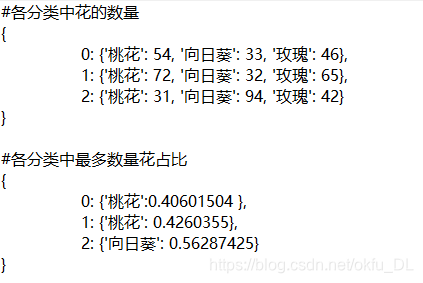
从训练结果可以看出,聚类效果并不好。应该是样本太少,而特征又稀疏(有像素点直接组成的特征)。
优化方案:
1.增加大量训练样本。
2.用CNN对图像进行特征提取。
事实上,如果选择方案一,则需要的样本可能是无穷大。那么,果断选择方案二。
VGG16特征提取。
下载vgg16的imgnet预训练参数,选择不带dense层的。因为如果带dense层会造成问题。若待分类样本在imgnet的1000个分类中,则结果就是vgg16的预测结果,可以直接选取最大值得index得到分类结果,聚类就显得毫无意义;若待分类样本不在这1000个分类中,则dense后的结果会有偏差。
参数下载地址(https://github.com/fchollet/deep-learning-models)
下载后模型默认保存在C盘的用户的.keras文件加下,例如weights_path = r'C:/Users/admin/.keras/models/'
filename: features.py
from vgg16 import VGG16
weights_path = r'C:/Users/admin/.keras/models/'


def get_feature(x):

    model = VGG16()
    model.load_weights(weights_path + 'vgg16_weights_tf_dim_ordering_tf_kernels_notop.h5')
    features = model.predict(x, batch_size=32, verbose=1)
    K.clear_session()
	return features
filename:vgg16.py
from keras.models import Model
from keras.layers import Flatten
from keras.layers import Input
from keras.layers import Conv2D
from keras.layers import MaxPooling2D


def VGG16():

    input_shape = (224,224,3)
    img_input = Input(shape=input_shape)
    x = Conv2D(64, (3, 3), activation='relu', padding='same', name='block1_conv1')(img_input)
    x = Conv2D(64, (3, 3), activation='relu', padding='same', name='block1_conv2')(x)
    x = MaxPooling2D((2, 2), strides=(2, 2), name='block1_pool')(x)

    # Block 2
    x = Conv2D(128, (3, 3), activation='relu', padding='same', name='block2_conv1')(x)
    x = Conv2D(128, (3, 3), activation='relu', padding='same', name='block2_conv2')(x)
    x = MaxPooling2D((2, 2), strides=(2, 2), name='block2_pool')(x)

    # Block 3
    x = Conv2D(256, (3, 3), activation='relu', padding='same', name='block3_conv1')(x)
    x = Conv2D(256, (3, 3), activation='relu', padding='same', name='block3_conv2')(x)
    x = Conv2D(256, (3, 3), activation='relu', padding='same', name='block3_conv3')(x)
    x = MaxPooling2D((2, 2), strides=(2, 2), name='block3_pool')(x)

    # Block 4
    x = Conv2D(512, (3, 3), activation='relu', padding='same', name='block4_conv1')(x)
    x = Conv2D(512, (3, 3), activation='relu', padding='same', name='block4_conv2')(x)
    x = Conv2D(512, (3, 3), activation='relu', padding='same', name='block4_conv3')(x)
    x = MaxPooling2D((2, 2), strides=(2, 2), name='block4_pool')(x)

    # Block 5
    x = Conv2D(512, (3, 3), activation='relu', padding='same', name='block5_conv1')(x)
    x = Conv2D(512, (3, 3), activation='relu', padding='same', name='block5_conv2')(x)
    x = Conv2D(512, (3, 3), activation='relu', padding='same', name='block5_conv3')(x)
    x = MaxPooling2D((2, 2), strides=(2, 2), name='block5_pool')(x)

    x = Flatten(name='flatten')(x)
    model = Model(img_input,x)

    return model
Dense降维
从vgg16的结构可以看出,最后一层卷积池化层的输出形状为(7,7,512),拉伸后为25088维向量,对于som分类这个向量维度还是太高了。我们在这个特征后面添加一层dense层,使其长度降维256,那么问题来了,Dense层的参数如何确定呢?
思路:
1.选择随机化的初始参数
2.通过训练调整
方案1很明显不行,否决了。那么如何通过训练调整dense层参数呢?想到了一个很巧妙的办法。看图: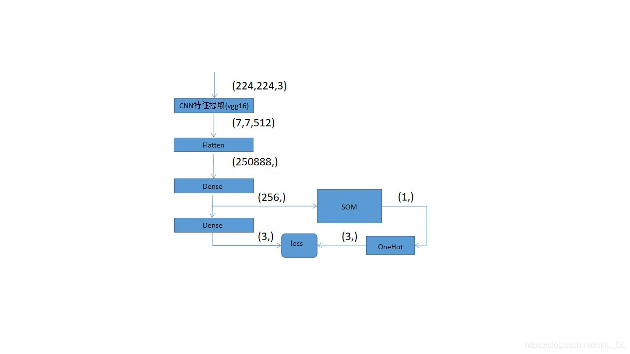
图中第一个dense层的256维向量作为som神经网络的输入特征;第二个dense层输出一个3维向量,我们将som神经网络得到的胜出类别转化为独热码后作为该输出向量的真值,以此计算损失函数,反向调整两个dense层的参数。
整个som的包含了两层dense层,其输入是flatten后的250888维向量。
最后放上修改后的som.py
filename:som.py
import tensorflow as tf
import numpy as np
from tqdm import tqdm  #一个进度条可以去掉
import re

inputshape = 25088

class SOM(object):

    _trained = False

    def __init__(self, m, n,dim, n_iterations=100, alpha=None, sigma=None):

        self._m = m
        self._n = n
        self.dim = dim

        if alpha is None:
            alpha = 0.3
        else:
            alpha = float(alpha)
        if sigma is None:
            sigma = max(m, n) / 2.0
        else:
            sigma = float(sigma)
        self._n_iterations = abs(int(n_iterations))
        self._centroid_grid = np.zeros(shape=(m,n))
        self.loaded_weights = None

        ##INITIALIZE GRAPH
        self._graph = tf.Graph()

        ##POPULATE GRAPH WITH NECESSARY COMPONENTS
        with self._graph.as_default():

            self._weightage_vects = tf.Variable(tf.random_normal(
                [m * n, dim],mean=0.5))

            self._location_vects = tf.constant(np.array(
                list(self._neuron_locations(m, n))))

            self._vect_input = tf.placeholder("float", [inputshape])   #输入的图片特征向量
            self._dense_input,self._output,self._dense_weights = self.dense(self._vect_input)
            self._iter_input = tf.placeholder("float")

            winner_index = tf.argmin(tf.sqrt(tf.reduce_sum(
                tf.square(tf.subtract(self._weightage_vects, tf.stack(
                    [self._dense_input[0] for i in range(m * n)]))), 1)),
                0)

            slice_input = tf.pad(tf.reshape(winner_index, [1]),
                                 np.array([[0, 1]]))
            self.winner_loc = tf.reshape(tf.slice(self._location_vects, slice_input,
                                          tf.constant(np.array([1, 2]),dtype=tf.int64)),
                                 [2])#等于self._location_vects[winner_index]
            print(self.winner_loc)

            learning_rate_op = tf.subtract(1.0, tf.divide(self._iter_input,
                                                  self._n_iterations))
            _alpha_op = learning_rate_op*alpha
            _sigma_op = sigma*learning_rate_op

            bmu_distance_squares = tf.reduce_sum(tf.square(tf.subtract(
                self._location_vects, tf.stack(
                    [self.winner_loc for i in range(m * n)]))), 1)#领域距离的平方向量

            neighbourhood_func = tf.exp(tf.negative(tf.divide(tf.cast(
                bmu_distance_squares, "float32"), tf.square(_sigma_op))))
            learning_rate_op = tf.multiply(_alpha_op, neighbourhood_func) #参数向量

            learning_rate_multiplier = tf.stack([tf.tile(tf.slice(
                learning_rate_op, np.array([i]), np.array([1])), [dim])
                for i in range(m * n)])

            weightage_delta = tf.multiply(
                learning_rate_multiplier,
                tf.subtract(tf.stack([self._dense_input[0] for i in range(m * n)]),
                            self._weightage_vects)) #增量矩阵
            new_weightages_op = tf.add(self._weightage_vects,
                                       weightage_delta)
            cross_entropy = tf.nn.sparse_softmax_cross_entropy_with_logits(logits=self._output,labels=[self.winner_loc[0]+self.winner_loc[1]])
            train_step = tf.train.ProximalGradientDescentOptimizer(learning_rate=_alpha_op).minimize(cross_entropy)
            self._training_op = tf.group(tf.assign(self._weightage_vects,
                                          new_weightages_op),train_step)

            ##INITIALIZE SESSION
            self._sess = tf.Session()

            ##INITIALIZE VARIABLES
            init_op = tf.global_variables_initializer()
            self._sess.run(init_op)

    def _neuron_locations(self, m, n):

        for i in range(m):
            for j in range(n):
                yield np.array([i, j])

    def train(self, input_vects):

        for iter_no in tqdm(range(self._n_iterations)):
            # Train with each vector one by one
            for input_vect in input_vects:
                # print(dense_vect.shape)
                self._sess.run(self._training_op,
                               feed_dict={self._vect_input: input_vect,
                                          self._iter_input: iter_no})

        # Store a centroid grid for easy retrieval later on
        self._locations = self._sess.run(self._location_vects)
        self._centroid_grid = self._sess.run(self._weightage_vects)
        self._dense_vects = self._sess.run(self._dense_weights)

        self._trained = True

    def save_weights(self,filename):
        need_save = [self._dense_vects,self._centroid_grid]
        if filename.endswith('npy'):
            np.save(filename,need_save)
        elif filename.endswith('txt'):
            with open(filename,'w') as f:
                f.write(str(need_save))
        elif filename.endswith('json'):
            import json
            with open(filename,'w') as f:
                json.dump(str(need_save),f)
        else:
            raise TypeError('cannot identify this type file')

    def load_weights(self,filename):
        if filename.endswith('npy'):
            weigths = np.load(filename)
        elif filename.endswith('txt'):
            with open(filename,'r') as f:
                weigths = eval(f.read())
        elif filename.endswith('json'):
            import json
            with open(filename,'r') as f:
                weigths = json.load(f)
        else:
            raise TypeError('cannot identify this type file')
        self.loaded_weights = weigths

    def predict(self,input_vects):
        if self.loaded_weights is None:
            raise RuntimeError('the weights not loaded')

        to_return = []
        locations =list(self._neuron_locations(self._m,self._n))
        dense_vects = np.dot(input_vects,self.loaded_weights[0])+0.1
        for vect in dense_vects:
            min_index = min([i for i in range(len(self.loaded_weights[1]))],
                            key=lambda x: np.linalg.norm(vect - self.loaded_weights[1][x]))
            to_return.append(locations[min_index])

        return to_return

    def evaluate(self,name_data,predict_data,classes):
        analysis = {}
        for i in range(self._m * self._n):
            each_class = {}
            for clas in set(classes):
                each_class[clas] = 0
            analysis[i] = each_class
        for name, result in zip(name_data, predict_data):

            idx = int(result[0]*self._n+result[1])
            analysis[idx][re.search("|".join(classes), name).group()] += 1

        score = {}
        for key, value in analysis.items():
            max_item = max(value.items(), key=lambda x: x[1])
            score[key] = {max_item[0]: max_item[1] / sum(value.values())}
        return analysis,score

    def dense(self,inputs_vect):
        inputs_vect = tf.expand_dims(inputs_vect,axis=0)
        w1 = tf.Variable(tf.random_normal([tf.shape(inputs_vect)[1], self.dim]))
        b1 = tf.constant(0.1,shape=[self.dim])
        z1 = tf.matmul(inputs_vect,w1)+b1
        a1 = tf.nn.relu(z1)

        w2 = tf.Variable(tf.random_normal([self.dim, self._m*self._n]))
        b2 = tf.constant(0.1,shape=[self._m*self._n])
        z2 = tf.matmul(a1,w2)+b2

        return a1,z2,w1
迭代1000轮,放上结果图
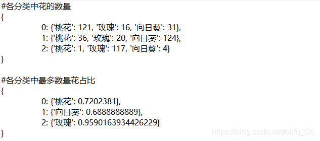
可见,分类效果已经初步达到。后期提高效果可以选择更好的CNN模型提取特征,或者多个CNN模型做特征融合。适当的调整学习率和迭代轮次,应该可以进一步提升分类结果。
好了,som图像分类介绍到这里,觉得有用的话,点个赞再走吧。