最近需要根据具体问题,识别数字,所以在kaggle上看了这个kernel
添加链接描述
- Introduction
- Data preparation
2.1 Load data
2.2 Check for null and missing values
2.3 Normalization
2.4 Reshape
2.5 Label encoding
2.6 Split training and valdiation set - CNN
3.1 Define the model
3.2 Set the optimizer and annealer
3.3 Data augmentation(数据增强) - Evaluate the model
4.1 Training and validation curves
4.2 Confusion matrix - Prediction and submition
5.1 Predict and Submit results
1. Introduction
This is a 5 layers Sequential Convolutional Neural Network for digits recognition trained on MNIST dataset. I choosed to build it with keras API (Tensorflow backend) which is very intuitive(直观的). Firstly, I will prepare the data (handwritten digits images) then i will focus on the CNN modeling and evaluation.
I achieved 99.671% of accuracy with this CNN trained in 2h30 on a single CPU (i5 2500k). For those who have a >= 3.0 GPU capabilites (from GTX 650 - to recent GPUs), you can use tensorflow-gpu with keras. Computation will be much much faster !!!
For computational reasons, i set the number of steps (epochs) to 2, if you want to achieve 99+% of accuracy set it to 30.
This Notebook follows three main parts:
- The data preparation
- The CNN modeling and evaluation
- The results prediction and submission
import pandas as pd
import numpy as np
import matplotlib.pyplot as plt
import matplotlib.image as mpimg
import seaborn as sns
%matplotlib inline

np.random.seed(2)

from sklearn.model_selection import train_test_split
from sklearn.metrics import confusion_matrix
import itertools

from keras.utils.np_utils import to_categorical # convert to one-hot-encoding
from keras.models import Sequential
from keras.layers import Dense, Dropout, Flatten, Conv2D, MaxPool2D
from keras.optimizers import RMSprop
from keras.preprocessing.image import ImageDataGenerator
from keras.callbacks import ReduceLROnPlateau


sns.set(style='white', context='notebook', palette='deep')

2. Data preparation
2.1 Load data
# Load the data
train = pd.read_csv("../input/train.csv")
test = pd.read_csv("../input/test.csv")

Y_train = train["label"]

# Drop 'label' column
X_train = train.drop(labels = ["label"],axis = 1)

# free some space
del train

g = sns.countplot(Y_train)

Y_train.value_counts()
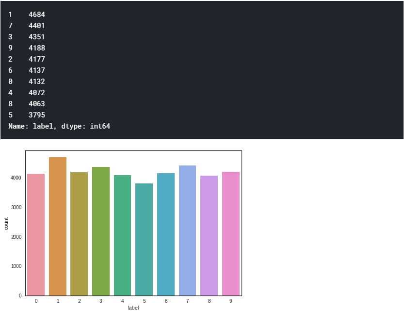
We have similar counts for the 10 digits.
2.2 Check for null and missing values
# Check the data
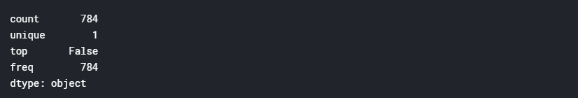
X_train.isnull().any().describe()
test.isnull().any().describe()
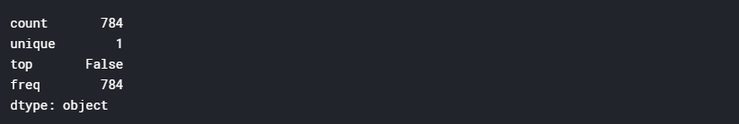
I check for corrupted images (missing values inside).

There is no missing values in the train and test dataset. So we can safely go ahead.
2.3 Normalization
We perform a grayscale normalization to reduce the effect of illumination’s(光照) differences.
Moreover the CNN converg faster on [0…1] data than on [0…255].

# Normalize the data
X_train = X_train / 255.0
test = test / 255.0
2.3 Reshape
# Reshape image in 3 dimensions (height = 28px, width = 28px , canal = 1)
X_train = X_train.values.reshape(-1,28,28,1)
test = test.values.reshape(-1,28,28,1)
Train and test images (28px x 28px) has been stock into pandas.Dataframe as 1D vectors of 784 values. We reshape all data to 28x28x1 3D matrices.
Keras requires an extra dimension in the end which correspond to channels. MNIST images are gray scaled so it use only one channel. For RGB images, there is 3 channels, we would have reshaped 784px vectors to 28x28x3 3D matrices.
2.5 Label encoding
# Encode labels to one hot vectors (ex : 2 -> [0,0,1,0,0,0,0,0,0,0])
Y_train = to_categorical(Y_train, num_classes = 10)
Labels are 10 digits numbers from 0 to 9. We need to encode these lables to one hot vectors (ex : 2 -> [0,0,1,0,0,0,0,0,0,0]).
2.6 Split training and valdiation set
# Set the random seed
random_seed = 2
# Split the train and the validation set for the fitting
X_train, X_val, Y_train, Y_val = train_test_split(X_train, Y_train, test_size = 0.1, random_state=random_seed)
I choosed to split the train set in two parts : a small fraction (10%) became the validation set which the model is evaluated and the rest (90%) is used to train the model.
Since we have 42 000 training images of balanced labels (see 2.1 Load data), a random split of the train set doesn’t cause some labels to be over represented in the validation set. Be carefull with some unbalanced dataset a simple random split could cause inaccurate evaluation during the validation.
To avoid that, you could use stratify = True option in train_test_split function (Only for >=0.17 sklearn versions).
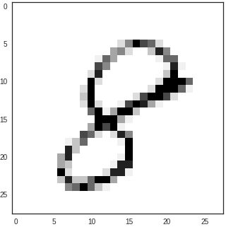
We can get a better sense for one of these examples by visualising the image and looking at the label.
# Some examples
g = plt.imshow(X_train[0][:,:,0])
3. CNN
3.1 Define the model
I used the Keras Sequential API, where you have just to add one layer at a time, starting from the input.
The first is the convolutional (Conv2D) layer. It is like a set of learnable filters. I choosed to set 32 filters for the two firsts conv2D layers and 64 filters for the two last ones. Each filter transforms a part of the image (defined by the kernel size) using the kernel filter. The kernel filter matrix is applied on the whole image. Filters can be seen as a transformation of the image.
The CNN can isolate features that are useful everywhere from these transformed images (feature maps).
The second important layer in CNN is the pooling (MaxPool2D) layer. This layer simply acts as a downsampling filter. It looks at the 2 neighboring pixels and picks the maximal value. These are used to reduce computational cost, and to some extent also reduce overfitting. We have to choose the pooling size (i.e the area size pooled each time) more the pooling dimension is high, more the downsampling is important.
Combining convolutional and pooling layers, CNN are able to combine local features and learn more global features of the image.
Dropout is a regularization method, where a proportion(比例)of nodes in the layer are randomly ignored (setting their wieghts to zero) for each training sample. This drops randomly a propotion (比例) of the network and forces the network to learn features in a distributed way. This technique also improves generalization and reduces the overfitting.
‘relu’ is the rectifier (activation function max(0,x). The rectifier activation function is used to add non linearity to the network.
The Flatten layer is use to convert the final feature maps into a one single 1D vector. This flattening step is needed so that you can make use of fully connected layers after some convolutional/maxpool layers. It combines all the found local features of the previous convolutional layers.
In the end i used the features in two fully-connected (Dense) layers which is just artificial an neural networks (ANN) classifier. In the last layer(Dense(10,activation=“softmax”)) the net outputs distribution of probability of each class.
# Set the CNN model
# my CNN architechture is In -> [[Conv2D->relu]*2 -> MaxPool2D -> Dropout]*2 -> Flatten -> Dense -> Dropout -> Out

model = Sequential()

model.add(Conv2D(filters = 32, kernel_size = (5,5),padding = 'Same',
                 activation ='relu', input_shape = (28,28,1)))
model.add(Conv2D(filters = 32, kernel_size = (5,5),padding = 'Same',
                 activation ='relu'))
model.add(MaxPool2D(pool_size=(2,2)))
model.add(Dropout(0.25))


model.add(Conv2D(filters = 64, kernel_size = (3,3),padding = 'Same',
                 activation ='relu'))
model.add(Conv2D(filters = 64, kernel_size = (3,3),padding = 'Same',
                 activation ='relu'))
model.add(MaxPool2D(pool_size=(2,2), strides=(2,2)))
model.add(Dropout(0.25))


model.add(Flatten())
model.add(Dense(256, activation = "relu"))
model.add(Dropout(0.5))
model.add(Dense(10, activation = "softmax"))
3.2 Set the optimizer and annealer(退火器)
Once our layers are added to the model, we need to set up a score function, a loss function and an optimisation algorithm.
We define the loss function to measure how poorly our model performs on images with known labels. It is the error rate between the oberved labels and the predicted ones. We use a specific form for categorical classifications (>2 classes) called the “categorical_crossentropy”.
The most important function is the optimizer. This function will iteratively improve parameters (filters kernel values, weights and bias of neurons …) in order to minimise the loss.
I choosed RMSprop (with default values), it is a very effective optimizer. The RMSProp update adjusts the Adagrad method in a very simple way in an attempt to reduce its aggressive(积极的), monotonically(单调) decreasing learning rate. We could also have used Stochastic Gradient Descent (‘sgd’) optimizer, but it is slower than RMSprop.
The metric function “accuracy” is used is to evaluate the performance our model. This metric function is similar to the loss function, except that the results from the metric evaluation are not used when training the model (only for evaluation).
# Define the optimizer
optimizer = RMSprop(lr=0.001, rho=0.9, epsilon=1e-08, decay=0.0)

# Compile the model
model.compile(optimizer = optimizer , loss = "categorical_crossentropy", metrics=["accuracy"])
In order to make the optimizer converge faster and closest to the global minimum of the loss function, i used an annealing method of the learning rate (LR).
The LR is the step by which the optimizer walks through the ‘loss landscape’. The higher LR, the bigger are the steps and the quicker is the convergence. However the sampling is very poor with an high LR and the optimizer could probably fall into a local minima.
Its better to have a decreasing learning rate during the training to reach efficiently the global minimum of the loss function.
To keep the advantage of the fast computation time with a high LR, i decreased the LR dynamically every X steps (epochs) depending if it is necessary (when accuracy is not improved).
With the ReduceLROnPlateau function from Keras.callbacks, i choose to reduce the LR by half if the accuracy is not improved after 3 epochs.
# Set a learning rate annealer
learning_rate_reduction = ReduceLROnPlateau(monitor='val_acc',
                                            patience=3,
                                            verbose=1,
                                            factor=0.5,
                                            min_lr=0.00001)

epochs = 1 # Turn epochs to 30 to get 0.9967 accuracy
batch_size = 86
3.3 Data augmentation
In order to avoid overfitting problem, we need to expand artificially our handwritten digit dataset. We can make your existing dataset even larger. The idea is to alter the training data with small transformations to reproduce the variations occuring when someone is writing a digit.
For example, the number is not centered The scale is not the same (some who write with big/small numbers) The image is rotated…
Approaches that alter the training data in ways that change the array representation while keeping the label the same are known as data augmentation techniques. Some popular augmentations people use are grayscales, horizontal flips, vertical flips, random crops, color jitters, translations, rotations, and much more.
By applying just a couple of these transformations to our training data, we can easily double or triple the number of training examples and create a very robust model.
The improvement is important :
- Without data augmentation i obtained an accuracy of 98.114%
- With data augmentation i achieved 99.67% of accuracy
# Without data augmentation i obtained an accuracy of 0.98114
#history = model.fit(X_train, Y_train, batch_size = batch_size, epochs = epochs,
#          validation_data = (X_val, Y_val), verbose = 2)

###############################################
# With data augmentation to prevent overfitting (accuracy 0.99286)

datagen = ImageDataGenerator(
        featurewise_center=False,  # set input mean to 0 over the dataset
        samplewise_center=False,  # set each sample mean to 0
        featurewise_std_normalization=False,  # divide inputs by std of the dataset
        samplewise_std_normalization=False,  # divide each input by its std
        zca_whitening=False,  # apply ZCA whitening
        rotation_range=10,  # randomly rotate images in the range (degrees, 0 to 180)
        zoom_range = 0.1, # Randomly zoom image
        width_shift_range=0.1,  # randomly shift images horizontally (fraction of total width)
        height_shift_range=0.1,  # randomly shift images vertically (fraction of total height)
        horizontal_flip=False,  # randomly flip images
        vertical_flip=False)  # randomly flip images


datagen.fit(X_train)
For the data augmentation, i choosed to :
- Randomly rotate some training images by 10 degrees
- Randomly Zoom by 10% some training images
- Randomly shift images horizontally by 10% of the width
- Randomly shift images vertically by 10% of the height
I did not apply a vertical_flip nor horizontal_flip since it could have lead to misclassify symetrical numbers such as 6 and 9.
Once our model is ready, we fit the training dataset .
# Fit the model
history = model.fit_generator(datagen.flow(X_train,Y_train, batch_size=batch_size),
                              epochs = epochs, validation_data = (X_val,Y_val),
                              verbose = 2, steps_per_epoch=X_train.shape[0] // batch_size
                              , callbacks=[learning_rate_reduction])

4. Evaluate the model
4.1 Training and validation curves
# Plot the loss and accuracy curves for training and validation
fig, ax = plt.subplots(2,1)
ax[0].plot(history.history['loss'], color='b', label="Training loss")
ax[0].plot(history.history['val_loss'], color='r', label="validation loss",axes =ax[0])
legend = ax[0].legend(loc='best', shadow=True)

ax[1].plot(history.history['acc'], color='b', label="Training accuracy")
ax[1].plot(history.history['val_acc'], color='r',label="Validation accuracy")
legend = ax[1].legend(loc='best', shadow=True)
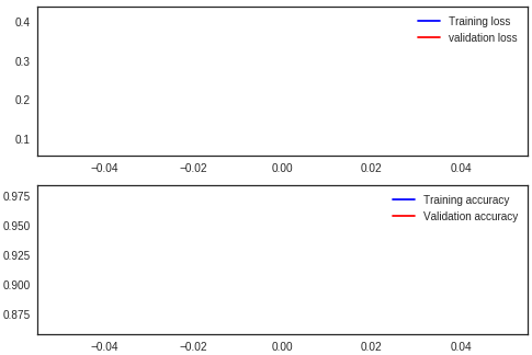
The code below is for plotting loss and accuracy curves for training and validation. Since, i set epochs = 2 on this notebook . I’ll show you the training and validation curves i obtained from the model i build with 30 epochs (2h30)
The model reaches almost 99% (98.7+%) accuracy on the validation dataset after 2 epochs. The validation accuracy is greater than the training accuracy almost evry time during the training. That means that our model dosen’t not overfit the training set.
Our model is very well trained !!!
4.2 Confusion matrix
Confusion matrix can be very helpfull to see your model drawbacks.
I plot the confusion matrix of the validation results.
# Look at confusion matrix

def plot_confusion_matrix(cm, classes,
                          normalize=False,
                          title='Confusion matrix',
                          cmap=plt.cm.Blues):
    """
    This function prints and plots the confusion matrix.
    Normalization can be applied by setting `normalize=True`.
    """
    plt.imshow(cm, interpolation='nearest', cmap=cmap)
    plt.title(title)
    plt.colorbar()
    tick_marks = np.arange(len(classes))
    plt.xticks(tick_marks, classes, rotation=45)
    plt.yticks(tick_marks, classes)

    if normalize:
        cm = cm.astype('float') / cm.sum(axis=1)[:, np.newaxis]

    thresh = cm.max() / 2.
    for i, j in itertools.product(range(cm.shape[0]), range(cm.shape[1])):
        plt.text(j, i, cm[i, j],
                 horizontalalignment="center",
                 color="white" if cm[i, j] > thresh else "black")

    plt.tight_layout()
    plt.ylabel('True label')
    plt.xlabel('Predicted label')

# Predict the values from the validation dataset
Y_pred = model.predict(X_val)
# Convert predictions classes to one hot vectors
Y_pred_classes = np.argmax(Y_pred,axis = 1)
# Convert validation observations to one hot vectors
Y_true = np.argmax(Y_val,axis = 1)
# compute the confusion matrix
confusion_mtx = confusion_matrix(Y_true, Y_pred_classes)
# plot the confusion matrix
plot_confusion_matrix(confusion_mtx, classes = range(10))
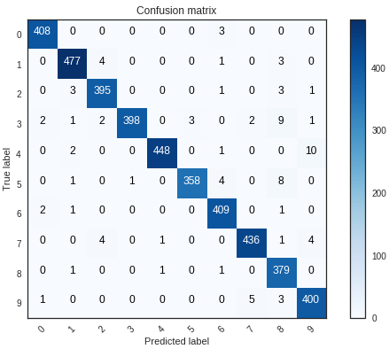
Here we can see that our CNN performs very well on all digits with few errors considering the size of the validation set (4 200 images).
However, it seems that our CNN has some little troubles with the 4 digits, hey are misclassified as 9. Sometime it is very difficult to catch the difference between 4 and 9 when curves are smooth.
Let’s investigate for errors.
I want to see the most important errors . For that purpose i need to get the difference between the probabilities of real value and the predicted ones in the results.
# Display some error results

# Errors are difference between predicted labels and true labels
errors = (Y_pred_classes - Y_true != 0)

Y_pred_classes_errors = Y_pred_classes[errors]
Y_pred_errors = Y_pred[errors]
Y_true_errors = Y_true[errors]
X_val_errors = X_val[errors]

def display_errors(errors_index,img_errors,pred_errors, obs_errors):
    """ This function shows 6 images with their predicted and real labels"""
    n = 0
    nrows = 2
    ncols = 3
    fig, ax = plt.subplots(nrows,ncols,sharex=True,sharey=True)
    for row in range(nrows):
        for col in range(ncols):
            error = errors_index[n]
            ax[row,col].imshow((img_errors[error]).reshape((28,28)))
            ax[row,col].set_title("Predicted label :{}\nTrue label :{}".format(pred_errors[error],obs_errors[error]))
            n += 1

# Probabilities of the wrong predicted numbers
Y_pred_errors_prob = np.max(Y_pred_errors,axis = 1)

# Predicted probabilities of the true values in the error set
true_prob_errors = np.diagonal(np.take(Y_pred_errors, Y_true_errors, axis=1))

# Difference between the probability of the predicted label and the true label
delta_pred_true_errors = Y_pred_errors_prob - true_prob_errors

# Sorted list of the delta prob errors
sorted_dela_errors = np.argsort(delta_pred_true_errors)

# Top 6 errors
most_important_errors = sorted_dela_errors[-6:]

# Show the top 6 errors
display_errors(most_important_errors, X_val_errors, Y_pred_classes_errors, Y_true_errors)
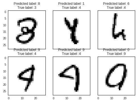
The most important errors are also the most intrigues(诡计).
For those six case, the model is not ridiculous. Some of these errors can also be made by humans, especially for one the 9 that is very close to a 4. The last 9 is also very misleading, it seems for me that is a 0.
# predict results
results = model.predict(test)

# select the indix with the maximum probability
results = np.argmax(results,axis = 1)

results = pd.Series(results,name="Label")

##################
submission = pd.concat([pd.Series(range(1,28001),name = "ImageId"),results],axis = 1)

submission.to_csv("cnn_mnist_datagen.csv",index=False)