机器学习基石笔记（二）：学会说 是/否

Lecture 2: Learning to Answer Yes/No

Perceptron Hypothesis Set

For $x = (x_1 ,x_2 ,··· ,x_d )$ ‘features of sample’, compute a weighted ‘score’( $\sum_{i=1}^{d}w_ix_i>threshold$)
and approve credit if score>threshold, deny credit if score>threshold and ignore the equals.
$Y:\{+1, -1\}$:
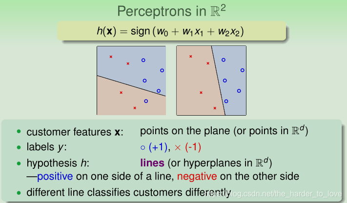
$h(x)=sign((\sum_{i=1}^{d}w_ix_i)-threshold) \stackrel{w_0 = -threshold, x_0 = +1}{\xlongequal{\quad\quad\quad\quad\quad\quad\quad}} sign((\sum_{i=1}^{d}w_ix_i)+w_0*x_0) \\ = sign((\sum_{i=0}^{d}w_ix_i)) = sign(w^Tx)$
called ‘perceptron’ hypothesis historically

Perceptrons in $R^2$

perceptrons（感知器） ⇔ linear (binary) classifiers

Fun Time

Consider using a perceptron to detect spam messages.
Assume that each email is represented by the frequency of keyword
occurrence, and output +1 indicates a spam. Which keywords below
shall have large positive weights in a good perceptron for the task?
1. coffee, tea, hamburger, steak
2. free, drug, fantastic, deal   $\checkmark$
3. machine, learning, statistics, textbook
4. national, Taiwan, university, coursera

Explanation
垃圾邮件常含"免费",’'打折","好消息"等词。

Perceptron Learning Algorithm (PLA)

PLA算法就是要在Perceptrons(Perceptron Hypothesis Set)找到合适的Perceptron，而Perceptron由 $w$决定，即找到合适 $w$，使样本完全分开。

Cyclic PLA

Cyclic PLA算法如下所示
（1）初始化 $w​$-> $w_0​$
（2）更新 $w​$
  For t = 0,1,…
    find a mistake of $w_t​$ called ( $x_{n(t)}​$, $y_{n(t)}​$)
       $sign(w_t^Tx_{n(t)}) \ne y_{n(t)}​$

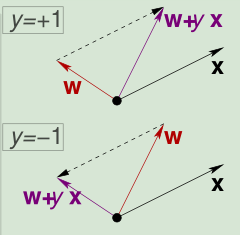
    correct the mistake by
       $w_{(t+1)} ← w_t + y_{n(t)}x_{n(t)}​$

  … until no more mistakes
  return last w (called $w_{PLA}​$ ) as g

PLA算法的精髓在于找到与感知器分类不正确的点，然后通过不正确的点修正感知器，直到所有的样本点分类正确。
修正公式： $w_{(t+1)} ← w_t + y_{n(t)}x_{n(t)}​$
修正图示：

Fun Time

Let’s try to think about why PLA may work.
Let n = n(t), according to the rule of PLA below, which formula is true?
$sign(w_t^Tx_{n}) \ne y_{n}，\quad w_{(t+1)} ← w_t + y_{n}x_{n}$
1.  $w_{t+1}^Tx_{n} = y_{n}$
2.  $sign(w_{t+1}^Tx_{n}) = y_{n}$
3.  $y_{n}w_{t+1}^Tx_{n} \geq y_{n}w_{t}^Tx_{n}$   $\checkmark$
4.  $y_{n}w_{t+1}^Tx_{n} < y_{n}w_{t}^Tx_{n}​$

Explanation
经过( $x_{n}$, $y_{n}$)更新后， $w_t$到 $w_{t+1}$的变化
由于感知器是相对修正( $\Delta w = y_{n}x_{n}$)，修正后不一定就能将( $x_{n}$, $y_{n}$)分类正确。

$y_{n}w_{t+1}^Tx_{n} - y_{n}w_{t}^Tx_{n} = (w_{t+1}^T-w_{t}^T)y_{n}x_{n} = x_{n}^Ty_{n}^Ty_{n}x_{n} \stackrel{y_{n}^Ty_{n}= +1}{\xlongequal{\quad\quad\quad}} x_{n}^Tx_{n} \ge 0​$

Guarantee of PLA

Linear Separability

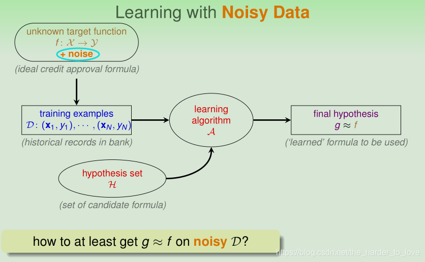
if PLA halts (i.e. no more mistakes), (necessary condition) D allows some w to make no mistake call such D linear separable.

linear separable $D$ ⇔ exists perfect $\mathbf{w_f}$ such that $sign(w_f^Tx_{n}) = y_{n}​$

感知器的修正

Fun Time中我们推导出感知器每次修正， $y_{n}w_{t+1}^Tx_{n} \ge y_{n}w_{t}^Tx_{n}$, $w_t$就会向 $w_f$逼近。
我们计算 $\Delta w_f^Tw_{t+1}​$再次确认下
$\because w_f \ is \ perfect \ for \ x_n \\ \therefore y_{n(t)}w_t^Tx_{n(t)} \ge \mathop{min}\limits_n \, y_{n(t)}w_t^Tx_{n(t)} > 0 \\ \mathbf{w_t^Tw_{n(t)} \uparrow} \ by \ updating \ with \ any \ (x_{n(t)}, y_{n(t)}) \\ \begin{aligned} \mathbf{w}_{f}^{T} \mathbf{w}_{t+1} &= \mathbf{w}_{f}^{T}\left(\mathbf{w}_{t}+y_{n(t)} \mathbf{x}_{n(t)}\right) \\ & \geq \mathbf{w}_{f}^{T} \mathbf{w}_{t}+\min _{n} y_{n} \mathbf{w}_{f}^{T} \mathbf{x}_{n} \\ &>\mathbf{w}_{f}^{T} \mathbf{w}_{t}+0 \end{aligned}$

感知器每次修正， $\mathbf{w}_{f}^{T} \mathbf{w}_{t+1} > \mathbf{w}_{f}^{T} \mathbf{w}_{t}​$， $w_t​$是在向 $w_f​$逼近。

但是我们希望的逼近是夹角的逼近，而不是数值的增大。计算 $\Delta||w_t||^2​$。

$\begin{aligned} \left\|\mathbf{w}_{t+1}\right\|^{2} &=\left\|\mathbf{w}_{t}+y_{n(t)} \mathbf{x}_{n(t)} \right\|^{2} \\ &=\left\|\mathbf{w}_{t}\right\|^{2}+2 y_{n(t)} \mathbf{w}_{t}^{T} \mathbf{x}_{n(t)}+\left\|y_{n(t)} \mathbf{x}_{n(t)}\right\|^{2} \\ 又 \ \operatorname{sign} & \left(\mathbf{w}_{t}^{T} \mathbf{x}_{n(t)}\right) \neq y_{n(t)} \Leftrightarrow y_{n(t)} \mathbf{w}_{t}^{T} \mathbf{x}_{n(t)} \leq 0 \\ & \leq\left\|\mathbf{w}_{t}\right\|^{2}+0+\left\|y_{n(t)} \mathbf{x}_{n(t)}\right\|^{2} \\ & \leq\left\|\mathbf{w}_{t}\right\|^{2}+\max _{n}\left\|y_{n} \mathbf{x}_{n}\right\|^{2} \\ & \leq\left\|\mathbf{w}_{t}\right\|^{2}+\max _{n}\left\| \mathbf{x}_{n}\right\|^{2} \end{aligned}$
最大增长不会超过 $\mathop{max} \limits_{n}\left\|\mathbf{x}_{n}\right\|^{2}​$

实际上 $w_0=0$，在T次修正后 $\cos\theta=\frac{\mathbf{w}_{f}^{T}}{\left\|\mathbf{w}_{f}\right\|} \frac{\mathbf{w}_{T}}{\left\|\mathbf{w}_{T}\right\|} \geq \sqrt{T} \cdot constant​$
证明:
$R^2 = \max _{n} \|\mathbf{x}_{n}\|^{2} \quad \rho = \frac{\min \limits _{n} y_{n} \mathbf{w}_{f}^{T} x_n}{\mathbf{\| w_f \|}} \\ \\ \because \mathbf{w_0 = 0} \quad \mathbf{w}_{f}^{T}\mathbf{w}_{T} \geq T\min \limits _{n} y_{n} \mathbf{w}_{f}^{T} \mathbf{x}_{n} \quad \left\|\mathbf{w}_{T}\right\|^{2} \leq T\max \limits _{n}\left\| \mathbf{x}_{n}\right\|^{2} \\ cos\theta=\frac{\mathbf{w}_{f}^{T}}{\left\|\mathbf{w}_{f}\right\|} \frac{\mathbf{w}_{T}}{\left\|\mathbf{w}_{T}\right\|} = \frac{1}{\left\|\mathbf{w}_{f}\right\|} \frac{\mathbf{w}_{f}^{T} \mathbf{w}_{T}}{\left\|\mathbf{w}_{T}\right\|} = \frac{1}{\left\|\mathbf{w}_{f}\right\|} \frac{T\min \limits _{n} y_{n} \mathbf{w}_{f}^{T} \mathbf{x}_{n}}{\sqrt{T}\sqrt{\max \limits _{n}\left\| \mathbf{x}_{n}\right\|^{2}}} \geq \sqrt{T}\frac{\rho}{R} \\ \therefore \cos\theta=\frac{\mathbf{w}_{f}^{T}}{\left\|\mathbf{w}_{f}\right\|} \frac{\mathbf{w}_{T}}{\left\|\mathbf{w}_{T}\right\|} \geq \sqrt{T} \cdot constant,\, 其中\, constant = \frac{\rho}{R}$

Fun Time

Let’s upper-bound T, the number of mistakes that PLA ‘corrects’.
$Define \, R^2 = \max _{n} \|\mathbf{x}_{n}\|^{2} \quad \rho = \frac{\min \limits _{n} y_{n} \mathbf{w}_{f}^{T} x_n}{\mathbf{\| w_f \|}}$

We want to show that $T \leq \square$. Express the upper bound $\square$ by the two terms above.
1 $\frac{R}{\rho}$
2 $\frac{R^2}{\rho^2}$   $\checkmark$
3 $\frac{R}{\rho^2}$
4 $\frac{\rho^2}{R^2}$


Explanation
$\sqrt{T}\frac{\rho}{R} \leq \frac{\mathbf{w}_{f}^{T}}{\left\|\mathbf{w}_{f}\right\|} \frac{\mathbf{w}_{T}}{\left\|\mathbf{w}_{T}\right\|} = cos\theta\leq 1 \\ \therefore T \geq \frac{\rho^2}{R^2}$

Non-Separable Data

More about PLA

保证
数据线性可分，存在一个感知器能使数据完全分开。

过程
通过一次次修正，更新感知器的参数。

结果
最终会达到完全可分，不知道会更新多少次。

Pocket PLA

假设数据存在噪音(noise)，线性不可分，此时我们想得到一个大致完全分类的感知器。
Pocket PLA：modify PLA algorithm (black lines) by keeping best weights in pocket
（1）初始化 $w$-> $w_0$
（2）更新 $w$
  For t = 0,1,…
    find a (random) mistake of $w_t$ called ( $x_{n(t)}$, $y_{n(t)}$)
       $sign(w_t^Tx_{n(t)}) \ne y_{n(t)}$

    correct the mistake by
       $w_{(t+1)} ← w_t + y_{n(t)}x_{n(t)}​$

    if $w_ {t+1}​$ makes fewer mistakes than $\hat{\mathbf{w}}​$, replace $\hat{\mathbf{w}}​$ by $w_ {t+1}​$
       $w_{(t+1)} ← w_t + y_{n(t)}x_{n(t)}​$

  … until engough iterations
  return $\hat{\mathbf{w}}$ (called $w_{Pocket}$ ) as g

Pocket PLA算法：
  按照PLA一样更新 $w_{t}​$的值，但是用一个Pocket(​ $\hat{\mathbf{w}}​$)存储当前犯错误最少的感知器。
  当执行一定时间或者更新次数，返回当前​ $\hat{\mathbf{w}}​$。

Fun Time

Should we use pocket or PLA?
Since we do not know whether D is linear separable in advance, we may decide to just go with pocket instead of PLA. If D is actually linear separable, what’s the difference between the two?
1 pocket on D is slower than PLA   $\checkmark$
2 pocket on D is faster than PLA
3 pocket on D returns a better g in approximating f than PLA
4 pocket on D returns a worse g in approximating f than PLA

Explanation
如果数据线性可分，PLA和Pocket PLA结果一样，获得一个将数据完全分类（no mistakes）的感知器；
但是Pocket PLA会慢些，主要原因是每一轮，需要检查犯错的个数；其次与当前最优感知器比较，替换也会耗费一些时间。

Summary

讲义总结

Perceptron Hypothesis Set
  感知器假设集是多维空间的超平面

Perceptron Learning Algorithm (PLA)
   $sign(w_t^Tx_{n(t)}) \ne y_{n(t)}​$， $w_{(t+1)} \leftarrow w_t + y_{n(t)}x_{n(t)}​$
   $g \leftarrow w_T ​$

Guarantee of PLA
  若数据集线性可分，则使用PLA算法，找一个完全分类的感知器。

Non-Separable Data
  若数据集线性不可分，则使用Pocket PLA算法，找一个较好的感知器。
  Pocket PLA算法按照PLA一样更新 $w_{t}$的值，但是用一个Pocket( $\hat{\mathbf{w}}$)存储当前犯错误最少的感知器。
   $g \leftarrow \hat{\mathbf{w}}$

PLA $A$ takes linear separable $D$ and perceptrons H to get hypothesis g

参考文献

《Machine Learning Foundations》(机器学习基石)—— Hsuan-Tien Lin (林轩田)