setwd("E:/08_cooperation/07_X-lab/06-Crosstalk/Aadapter_primer")
# 读取lane01.txt,并对其按列进行相加处理,然后对列进行进行命名
d1=read.table("lane01.txt",header = FALSE,sep = ",")
cyc001=d1$V3+d1$V4+d1$V5+d1$V6
d1=cbind(d1,cyc001)
names(d1)=c("cyc001x","cyc001y","cyc001A","cyc001T","cyc001C","cyc001G","cyc001")
# 读取lane06.txt,并对其按列进行相加处理,然后对列进行进行命名
d2=read.table("lane06.txt",header = FALSE,sep = ",")
cyc001=d2$V3+d2$V4+d2$V5+d2$V6
d2=cbind(d2,cyc001)
names(d2)=c("cyc001x","cyc001y","cyc001A","cyc001T","cyc001C","cyc001G","cyc001")
head(d1)
cyc001x cyc001y cyc001A cyc001C cyc001G cyc001T cyc001
1 29.20 2.94 798 697 831 1322 3648
2 83.36 3.51 1379 575 455 3185 5594
3 121.10 2.82 1049 377 371 4249 6046
4 150.12 2.42 1093 1317 1275 1157 4842
5 159.20 3.58 1124 993 428 5124 7669
6 194.29 2.63 1178 1007 372 1328 3885
head(d2)
cyc001x cyc001y cyc001A cyc001C cyc001G cyc001T cyc001
1 37.57 3.14 2374 6680 1337 1501 11892
2 108.90 3.11 3469 3720 528 5688 13405
3 270.51 4.34 6710 1868 1039 4087 13704
4 136.98 4.11 1753 11892 873 1656 16174
5 142.14 3.93 1677 2732 1366 3399 9174
6 234.00 4.00 1657 7318 727 1524 11226
#载入plyr包
library(plyr)
listA<-list()
listA[[1]] <- data.frame(t(d1$cyc001A))
listA[[2]] <- data.frame(t(d2$cyc001A))
A<-t(rbind.fill(listA))
colnames(A)<-c("lane01_A","lane06_A")
write.table(A,file="intsfile_A.txt")
listT<-list()
listT[[1]]<-data.frame(t(d1$cyc001T))
listT[[2]]<-data.frame(t(d2$cyc001T))
T<-t(rbind.fill(listT))
colnames(T)<-c("lane01_T","lane06_T")
write.table(T,file="intsfile_T.txt")
listC <- list()
listC[[1]] <- data.frame(t(d1$cyc001C))
listC[[2]] <- data.frame(t(d2$cyc001C))
C<- t(rbind.fill(listC))
colnames(C) <-c("lane01_C","lane06_C")
write.table(C,file="intsfile_C.txt")
listG <- list()
listG[[1]] <- data.frame(t(d1$cyc001G))
listG[[2]] <- data.frame(t(d2$cyc001G))
G<- t(rbind.fill(listG))
colnames(G) <-c("lane01_G","lane06_G")
write.table(G,file="intsfile_G.txt")
listCyc <- list()
listCyc[[1]] <- data.frame(t(d1$cyc001))
listCyc[[2]] <- data.frame(t(d2$cyc001))
ATCG<- t(rbind.fill(listCyc))
colnames(ATCG) <-c("lane01","lane06")
write.table(ATCG,file="intsfile_ATCG.txt")
list.files()
[1] "201811271857_lane06_8mix_10A_100B2" "201904171659_B028___Lane01_03_05"
[3] "intsfile_A.txt" "intsfile_ATCG.txt"
[5] "intsfile_C.txt" "intsfile_G.txt"
[7] "intsfile_T.txt" "lane01.txt"
[9] "lane06.txt"
library(wordcloud2)
library(gcookbook)
library(ggplot2)
library(reshape2)
data=read.table("intsfile_ATCG.txt",header = T)
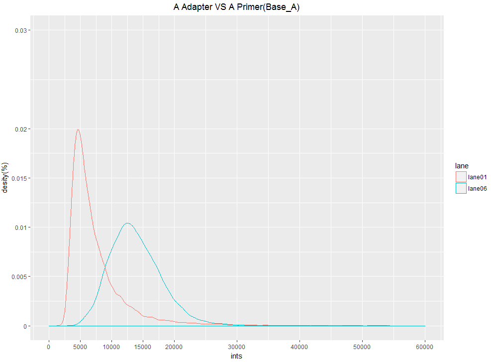
data1=melt(data,variable.name="lane",value.name="ints")
ggplot(data1,aes(x=ints,colour=lane))+geom_density(adjust=1)+ggtitle("A Adapter VS A Primer(Base_A)")+theme(plot.title=element_text(size=rel(1.2),hjust = 0.5,family="Times"))+scale_x_continuous(limits = c(0,60000),breaks = c(0,5000,10000,15000,20000,30000,40000,50000,60000))+scale_y_continuous("desity(%)",limits = c(0,0.0003),breaks = c(0.00000,0.00005,0.00010,0.00015,0.00020,0.00030),labels = c(0.00000,0.00005,0.00010,0.00015,0.00020,0.00030)*100)