支持向量机-人脸识别

引入所需函数和包

from time import time
import logging
import matplotlib.pyplot as plt
from sklearn.model_selection import train_test_split
from sklearn.datasets import fetch_lfw_people
from sklearn.model_selection import GridSearchCV
from sklearn.metrics import classification_report
from sklearn.metrics import confusion_matrix
from sklearn.decomposition import PCA
from sklearn.svm import SVC

第一步，加载数据集

# 数据集下载到了本地下载文件下中
lfw_people = fetch_lfw_people(min_faces_per_person=70, resize=0.4)
# n_sample实例的数量
n_sample,h,w=lfw_people.images.shape

print(lfw_people.images.shape)---------------------(1288, 50, 37)

第二步，划分测试集和训练集，获取label，和图片维度

X=lfw_people.data
# 每张图片的维度,1代表列数
n_features=X.shape[1]
# 返回数据集对应的label
y=lfw_people.target
target_names=lfw_people.target_names
# 总共的类别
n_classes=target_names.shape[0]
print(n_sample)
print(n_features)
print(n_classes)
print(n_features)
print(y,len(y))
X_train,X_test,y_train,y_test=train_test_split(X,y,test_size=0.25)

第三步，降低图片维度

n_components=150
t0=time()
# 降维
# n_components：这个参数可以帮我们指定希望PCA降维后的特征维度数目
# whiten ：判断是否进行白化，就是对降维后的数据的每个特征进行归一化
pca=PCA(svd_solver='randomized',n_components=n_components,whiten=True).fit(X_train)
# 对人脸照片提取特征值
eigenfaces=pca.components_.reshape((n_components,h,w))
print(time()-t0)
t0=time()
X_train_pca=pca.transform(X_train)
X_test_pca=pca.transform(X_test)
print(time()-t0)
t0=time()
# 对这两个参数尝试不同的值
# 多少的比例的特征值会使用
param_grid={'C':[1e3,5e3,1e4,5e4,1e5],
            'gamma':[0.0001,0.0005,0.001,0.005,0.01,0.1],}
# C越大，相当于惩罚松弛变量，希望松弛变量接近0，即对误分类的惩罚增大，
# 趋向于对训练集全分对的情况，这样对训练集测试时准确率很高，但泛化能力弱。
# C值小，对误分类的惩罚减小，允许容错，将他们当成噪声点，泛化能力较强。
# gamma ： ‘rbf’,‘poly’ 和‘sigmoid’的核函数参数。默认是’auto’，则会选择1/n_features

第四步，调用库函数训练

clf=GridSearchCV(SVC(kernel='rbf'),param_grid)
clf=clf.fit(X_train_pca,y_train)
print(time()-t0)
print(clf.best_estimator_)
t0=time()
y_pred=clf.predict(X_test_pca)
print(time()-t0)
print(classification_report(y_test,y_pred,target_names=target_names))
print(confusion_matrix(y_test,y_pred,labels=range(n_classes)))

第六步，画图显示结果

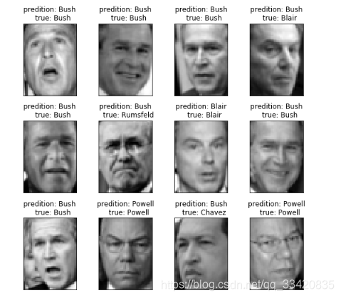
def plot_galley(images,titles,h,w,n_row=3,n_col=4):
    plt.figure(figsize=(1.8*n_col,2.4*n_row))
    plt.subplots_adjust(bottom=0,left=.01,right=.99,top=.90,hspace=.35)
    for i in range(n_row*n_col):
        plt.subplot(n_row,n_col,i+1)
        plt.imshow(images[i].reshape((h,w)),cmap=plt.cm.gray)
        plt.title(titles[i],size=12)
        plt.xticks(())
        plt.yticks(())
def title(y_pred,y_test,target_names,i):
    pred_name=target_names[y_pred[i]].rsplit(' ',1)[-1]
    true_name=target_names[y_test[i]].rsplit(' ',1)[-1]
    return ('predition: %s\n   true: %s'% (pred_name,true_name))
prediction_titles=[title(y_pred,y_test,target_names,i) for i in range(y_pred.shape[0])]
plot_galley(X_test,prediction_titles,h,w)
eigenface_titles=['eigenface %d' % i for i in range(eigenfaces.shape[0])]
plot_galley(eigenfaces,eigenface_titles,h,w)
plt.show()

显示结果：

支持向量机-人脸识别

猜你喜欢