This blog and the following blogs revolve around the topic about Digital Image Processing.
All the contents are from Hamed Sari-Sarraf.
这门课是学校开的一门关于图像处理的学习课程,课程内容较为宽大,本人根据学习内容归纳总结,可能有不对或不详之处,望指正。
Contact me: [email protected] , if necessary.
DL-Digital Image Processing-Summary
Day-1
Introduction
Artificial Intelligence (AI)
- Computer vision: sub-field of AI (Extract information from images)
- Image processing: sub-field of C-V
image -> IP -> image - machine learning (pattern recognition): sub-field of AI
data -> ML -> information
What skills are needed in AI?
- Mathematics
- Probability of statistics
- Programming (Python)
Tips: 这里讲的是一些老生常谈的东西,这门课讲的是什么?该具备的啥技能?
Image features
- BW(black and white):
- Three channels: RGB
Tips: 如果只承认灰度,对于一张图片而言,上面的每个像素点的取值范围都是0-255,因为每个像素点只有一种表示灰度的值,它是一个字节,八位。如果是将RGB组合进去的话,那么每个像素点,就可以囊括3个字节,或者变为3层组合。可以想象得到3个矩阵。
Type of image features
- Key points or interest points (Corners)
- Edges, Curves, Straight lines
- Patches
Tips: 要辨别一张图片,靠人眼很容易看出来,那么靠计算机呢?那么我们就得挖掘它的特征。特征有很多很多,就像上面呈现的。关键图点,边,曲线,直线,图块,都可以。
Why detect image features? (Good Effects)
- Color Calibration
- Image Stitching
- Computing Camere Pose
- 3D Scene Reconstruction
- Object Recognition
我们研究图像特征是为了做什么?它有什么帮助嘛?颜色校正(这里可以举例我们可以通过观察颜色确定一种花),图形拼接,相机定位(通过观察图片,确定照相者的位置),3D重构成像(你要拍很多很多的不同角度的照片哦),对了还有最普遍的一种,就是识别物体,这在无人驾驶领域很重要的哇。
What are “good” features?
- Repeatability
- Distinctiveness
- Locality
- Quantity
- Accuracy
- Efficiency
tips: 那么,什么是好的特征呢?假设有两幅图,第一幅是object(denote ),第二幅是scene(denote ),我们需要在 中找到 的位置。这里说的好的特征值的是,我们在选择特征的时候,要找重复的( 就是这个 具备的特征,能在 中找到,找到很多不要紧,至少要有吧,这里我是这么理解的),然后要有特性(这个不解释),局部性(就是即便是 中有被遮挡的部分,只要 中的某些局部特征仍然存在,那么在 中就可以找到对应位置),像准确率这种东西我也不解释了,对了,还有一个是高效(就是计算机在识别这些特征时一定要快,不然车就翻了)。
我们上面谈了那么多,那么我们学习深度学习之图像处理究竟是为了做什么呢?现在呢,这节课讨论的点就是:第一幅是object(denote ),第二幅是scene(denote ),我们需要在 中找到 的位置。并确定“相似程度”(我喜欢这么叫)?不过呢,我们先来补一补一些数学知识,再实战代码咯(matlab,python)。
Formula
What is correlation?
Before talking about the fomula, let’s learn something about it.
- Supposing there are two pictures, the first ( ) is called the scene, while the second( ) is called object (or pattern). Just as the following picture.
- Then we will define the Convolution and Correlation and interpret how do they intereact with each other.

我们确定object 与scene 。为了使操作使得结果看起来更舒适些,我们将 “放大”,然后把 贴上去,然后向右平移,平移完 后,再换 平移,直到将整个 平移完,在平移过程中,我们对 分别做了以下 Convolution 和 Correlation 操作。进行这两个操作是为了将其实例化,其实最终目的是为了判别 与 找到的位置的“相似程度”有多高。
以下操作均包含三个步骤:
- 像素点相乘
- 相加
- 移动
Convolution
Convolution (卷积函数,这么叫是直译过来的,其实要我理解是旋转的意思,你也看到了,将图片 转过来操作) between f and w is defined as:

Correlation
Correlation (相关性) between f and w is defined as:

Mathematically, correlation and convolution are not equal (concretely, the same), button practice they are quite similar.
这两个公式在数学上相似,严格定义却不同,我们移动 ,也就类似移动 ,但实际上很相似。
But then, how do we evaluate it?
Normalized Cross-Correlation(我们定义了这个公式用来衡量“相似程度”)
值的范围: ,1代表最相似,0代表最不相似,-1代表negative相似(老师举的例子是黑白图片盒白黑图片的相似程度为-1,是不是与颜色有关,这里没有深究); 代表 的均值, 代表与 吻合(大小)部分的均值。
About Coding
终于到了代码部分,matlab(octave)代码还是很简单的,至少很多集成的函数实现都是封装的,但是这里最麻烦的是关于照片的选取问题,因为纬度不同会导致很多问题。
这里我选择了下面三张图片500*300(按顺序)


close all;
clear;
%读取数据,这里就是加载三张图片
x1=imread('1.jpg');
x2=imread('2.jpg');
x3=imread('3.jpg');
x=[x1,x2,x3];%将三张图片合在一起
imshow(x)%画出来

template=x2;%确定模版,我喜欢说它是pattern,好吧,object。
figure;%确定一张面板
imshow(template)%将这个object画上去咯

c=normxcorr2(rgb2gray(template),rgb2gray(x));%这一步计算Normalized Cross-Correlation的值
figure,surf(c),shading flat %就是画画,surf曲面图

[ypeak,xpeak]=find(c==max(c(:))); %找到c值最大时的中心位置,记为peak值,峰值,这个是为了后续咱们为了标注用的
yoffSet=ypeak-size(template,1);%1代表行,2代表列,这是在找坐标位置
xoffSet=xpeak-size(template,2);%为了画出一个矩形

figure;%依旧确定一张面板

imshow(x);%画画咯
h=imrect(gca,[xoffSet+100,yoffSet+100,size(template,2)/1.5,size(template,1)/1.5]);%这里参数挺多的,但其实,gca应该是确定画的方式,后面一堆参数决定位置点
setColor(h,'r')%颜色
结果如下:


当然,这个课程还是有作业的,如何破坏这种机制,让它相似程度达不到1?
- 放大?
- 缩小?
- 旋转?
由于操作较为简单,这里就不给出具体结果了。这里只给出代码:
close all;
clear;

x1=imread('1.jpg');
x2=imread('2.jpg');
x3=imread('3.jpg');
x=[x1,x2,x3];
imshow(x)

template=x2;
rotang=input('Give a Rotation Angle (in degree) -> ');%增加部分
sca=input('Give a Scale factor -> ');%输入提示
template=imrotate(template,rotang,'bilinear','crop');%旋转角度
template=imresize(template,sca);%缩放大小
figure;
imshow(template)

c=normxcorr2(rgb2gray(template),rgb2gray(x));
figure,surf(c),shading flat

[ypeak,xpeak]=find(c==max(c(:)));
yoffSet=ypeak-size(template,1);
xoffSet=xpeak-size(template,2);

figure

imshow(x);
h=imrect(gca,[xoffSet+100,yoffSet+100,size(template,2)/1.5,size(template,1)/1.5]);
setColor(h,'r')
Day 2
- Three important properties for an object recognition algorithm
- Geometric transformation
- Edge detection
- Harris Corner detector
Tips: 这节课主要讲物体识别算法的三个重要属性,几何变形,edge探测,corner探测。
Three important properties
For an object recognition algorithm
- Translation (shift) invariant (移动不变性)
- Rotation invariant (旋转不变性)
- Scale invariant (缩放不变性)
- Photometric invariance (光度不变性)

Fig. Basic set of 2D planar transformations
| If changes(Y/N) | Orrientation | Length | Angles | Parallelism | Straightlines |
|---|---|---|---|---|---|
| translation | N | N | N | N | N |
| Euclidean | Y | N | N | N | N |
| Similarity | Y | Y | N | N | N |
| Affine | Y | Y | Y | N | N |
我们根据上节课的代码展示得出结论:
的大小缩放可能对在 中的图像识别造成影响,其实我们希望,即使是图像在经过这些操作后仍然可以在 中识别出来。那么,首先一个问题是,我们如何利用矩阵对 进行旋转,平移等操作呢?
Geometric transformation
几何变形。设我们有一张 图片(上面有一点 ),经过矩阵操作后,有一张 图片(上面对应点为 )。我们进行的操作是:
其中矩阵最后一列 是用来对点进行移动操作的,所以并未设置成参数。
其他操作如下图。

Edge detection
在深入研究 之前,我们先来学习一些图片预处理代码知识:
对于一张给定的”building1.JPG”图片。

我们进行以下操作:
>> x=imread('building1.JPG');%读入图片,存储以矩阵形式
>> whos
  Name        Size                Bytes  Class    Attributes

  x         480x640x3            921600  uint8

>> x=rgb2gray(x);%只留下灰度,一层,我们可以比较size
>> whos
  Name        Size              Bytes  Class    Attributes

  x         480x640            307200  uint8

>> imshow(x)%展示图片
得到灰度图片:

如果我们沿用 中 公式:
>> x=imread('building1.JPG');
>> x=rgb2gray(x);
>>
>> subplot(1,5,1);imshow(x)
>>
>> w1=[1,-1];
>> out1=conv2(x,w1,'same');%运用公式
>> subplot(1,5,2);imshow(out1,[])
>>
>> w2=[-1,1];
>> out2=conv2(x,w2,'same');
>> subplot(1,5,3);imshow(out2,[])
>>
>> w3=[1;-1];
>> out3=conv2(x,w3,'same');
>> subplot(1,5,4);imshow(out3,[])
>>
>> w4=[-1;1];
>> out4=conv2(x,w4,'same');
>> subplot(1,5,5);imshow(out4,[])
>>
我们会得到以下不同的图片:

这很有意思,不是吗?至少我们可以得出一个结论,昨天的 公式对图片起到了一个类似过滤(filter)作用。所以为了研究 ,(由于绘图麻烦,这次直接。。)板书如下:

(这张图片左上角是一张图片,提出问题如何找到edge;左下角是一个序列和一个
的过滤图,类似于
里的
,具体说明Tip1;然后右边是一个图像类似于
的函数图像和其一阶导,二阶导图像(科普点这里,当然与这内容没啥直接联系),具体说明Tip2)
Tip2:
先看Tip2,原因是这里说明了如何找到
,这个函数图像
并非对应着其左边的图,它说明的是一个序列图(所有像素点排成一行),然后我们对其一阶求导,图像如图所示,再求二阶导,图像类似如上:可能有人会疑问,二次求导不应该全是常数0么?这里只是为了解释突变现象的发生,确定
的发生,与一阶导最大值,或者说二阶导为0值时对应的
有关。
Tip1:
然后看Tip1,
类似一个过滤器,它的作用充当了一阶求导过程,先把
置于像素序列点之上,对应点相乘,再相加,值记录在
右端点对应位置下侧,然后向右不断移动
,直至出现不为0的点,这个点对应的位置就是
首次被探测到的位置。注意,无论
的维数是多少,都满足一点,其矩阵内部元素相加和为0,这样才能使得一阶求导在
图像上过滤值为0,而不是其他值,这样也正好满足了条件需求。
Harris Corner detector
如何利用计算机辨别
和
呢?这里重点
。

如上图,我们规定从左至右图片编号(1-5),对于这5张图片,我们各加了一个窗口,现在我们假定在这些窗口中看外面的图片(1-5)移动,对于 图片,我们看不出任何变化;对于有 的图片,我们可以看到图片在朝某个方向移动时,我们视线上的图片会发生改变;对于有 的图片,我们发现图片在朝任意方向移动时,我们视线上的图片都会发生改变。为了使这种操作更加数值化,我们引入 :
可以这样理解,我们研究的图片经过平移后,他们上的点与原始图形的差的平方和数值。
根据泰勒公式,我们对
展开前几项:
所以,
接着,将
代入原公式,我们可以得到:
针对上式,我们记作 , 其中我们要求 。
我们的最优化问题就变为,找到合适的 ,使得 最大。
即 合适的 , 。
Tips: 这里的要求 是为了使的 标准化,虽然 的作用是移动图形,但这里是相当于在笛卡尔坐标系中找到一个方向,找到方向后再确定具体数值移动位数。
然后我们怎样实例化呢?我的意思是说,如何通过数值比较来判断这张我们探测的图是否存在edge或者corner呢?
Answer:
我们通过计算 的特征值与与之对应的特征向量。当然我们重点看特征值 和 的大小:如果都小–>图像是flat的;如果一大一小–>图像是有edge的;如果都大–>图像是有corner的。
与此同时,我们插入窗口来找 或者 的位置:
其中 就是一个窗口函数(这里说的比较浅,只说它是用来确定位置的),具体图像:


Questions
上面的问题只是涉及到图像旋转与移动,那么当图像变大或者变小时,最终又会有怎样的结果呢?
关于本节课的code部分
用到图片如下:
building1.JPG

building2.JPG

还有一张tif格式图片6,这里不便给出
代码段1:
%这段代码的作用拟合几张图片,确定其中是否有edge或者corner
close all
clear

i{1}=zeros(64,64);
i{2}=zeros(64,64);
i{2}(33:64,:)=0.5;
i{3}=zeros(64,64);
i{3}(:,33:64)=0.5;
i{4}=i{2}+i{3};
i{4}(i{4}>0.5)=0;
i{5}=imrotate(i{4},30,'crop');

[I,y]=meshgrid(1:64,1:64);
win=exp(-((I-32).^2+(y-32).^2)/5); %Window Function

rng(20);
k=0.06;
for j=1:5
    I=imnoise(i{j},'gaussian',0.5,0.01);
    subplot(2,5,j); imshow(I,[]);
    [Ix,Iy]=imgradientxy(I,'sobel');
    Ix=win.*Ix;
    Iy=win.*Iy;
    subplot(2,5,j+5); plot(Ix,Iy,'go');
    xlabel('I_x'); ylabel('I_y');
    axis([-2 2 -2 2]); axis square; grid on; hold on
    II=[reshape(Ix,[64*64,1]),reshape(Iy,[64*64,1])];
    II=II-mean(II);
    M=cov(II)*(64*64-1);
    [V,D]=eig(M);
    LamR=D(2,2)/(D(1,1)+D(2,2));
    if LamR > 0.9
        quiver(0,0,V(1,2),V(2,2),'LineWidth',1)
    else
        quiver(0,0,V(1,1),V(2,1),'LineWidth',1)
        quiver(0,0,V(1,2),V(2,2),'LineWidth',1)
    end
    R=det(M)-k*trace(M)^2;
    title(['\lambda_1=',num2str(D(1,1),'%0.1f'),...
        ', \lambda_2=',num2str(D(2,2),'%0.1f'),', R=',num2str(R,'%0.1f')]);
end
结果:

其中R值也是衡量其中是否有edge或者corner的另一指标,当R值很小时,flat;当R值为负值时,edge;当R值为很大正值时,corner。
代码段2:
%%标记出corner位置
I=checkerboard(32);
corners = detectHarrisFeatures(I);
figure; imshow(I);
hold on
plot(corners.Location(:,1),corners.Location(:,2),'r*','LineWidth',2);
结果:

代码段3:
%%标记不同6的corner
I=rgb2gray(imread('digit6.tif'));
corners = detectHarrisFeatures(I);
figure; imshow(I);
hold on
plot(corners.Location(:,1),corners.Location(:,2),'r*','LineWidth',2);
I=imrotate(rgb2gray(imread('digit6.tif')),30,'bilinear','crop');
corners = detectHarrisFeatures(I);
figure; imshow(I);
hold on
plot(corners.Location(:,1),corners.Location(:,2),'r*','LineWidth',2);
I=imresize(rgb2gray(imread('digit6.tif')),6,'bilinear');
corners = detectHarrisFeatures(I);
figure; imshow(I);
hold on
plot(corners.Location(:,1),corners.Location(:,2),'r*','LineWidth',2);
结果:


代码段4:
%%不同building的corner位置
I=rgb2gray(imread('building1.jpg'));
corners = detectHarrisFeatures(I);
figure; imshow(I);
hold on
plot(corners.Location(:,1),corners.Location(:,2),'r*','LineWidth',2);
I=rgb2gray(imread('building2.jpg'));
corners = detectHarrisFeatures(I);
figure; imshow(I);
hold on
plot(corners.Location(:,1),corners.Location(:,2),'g*','LineWidth',2);
结果:


Day3
- Feature matching
- Scale-Invariant Features Transform (SIFI)
先吐槽一番,博客忘保存了,写了两波,心态有点炸。今天老师讲的内容挺少的,主要讲了特征匹配(原理和实现),概括性地讲了一点缩放不变性。
Feature matching
- feature detection
特征探测 - feature describing
A vector describing what the image “looks like” in a neighborhood around each detected feature.(放一个窗口在某一个特征上,观察其周围的邻居) - feature matching
特征匹配
特征匹配的目的是为了使的计算机能够辨别对于经过几何变换的图形之间的特征的映射。
举个栗子

如上,假设有一张蓝色正方形图片和一张旋转过的蓝色正方形图片,我们已经标记好上面的特征(corner)的位置,用 , , , ; , , , 表示,我们的目的是为了将两张图片上不同位置的特征用计算机匹配出来(我们当然知道这对人来说很容易,但计算机就要费一点功夫了,对了,首先要对这些特征向量化)。假设我们选定:
这些向量之间哪两个更相似呢?于是我们利用欧氏距离,选定最小的:
则, 与 更相似,即我们假设的 与 更相似。
现在,对应到具体的实践操作又是怎样的呢?
Code部分
利用图片:Day2中building1.JPG和building2.JPG
code1:利用Harris算法查找所有corner
%%
%%detectHarrisFeatures
close all
clear
I =rgb2gray(imread('building1.JPG'));%载入图像
corners=detectHarrisFeatures(I);
imshow(I);hold on;
plot(corners.selectStrongest(10000));%选取前10000个效果最好的
结果:

code2:过滤部分特征,根据邻居信息过滤
%%
%%extractFeatures-1
close all
clear
I=rgb2gray(imread('building1.JPG'));
corners = detectHarrisFeatures(I);
%Find and extract corner features
[features, valid_corners] = extractFeatures(I, corners);
figure; imshow(I); hold on
plot(valid_corners);
%%
%%extractFeatures-2
close all
clear
I = rgb2gray(imread('building1.JPG'));
points = detectSURFFeatures(I);
[features, valid_points] = extractFeatures(I, points);
figure; imshow(I); hold on;
plot(valid_points.selectStrongest(100),'showOrientation',true);
%%
%%extractFeatures-3
close all
clear
I = rgb2gray(imread('building1.JPG'));
regions = detectMSERFeatures(I);
[features, valid_points] = extractFeatures(I,regions,'Upright',true);%regions-upright
figure; imshow(I); hold on;
plot(valid_points,'showOrientation',true);
不同结果:


code3:匹配特征
%%
%%match Features-1
close all
clear
I1 = rgb2gray(imread('building1.JPG'));
I2 = rgb2gray(imread('building2.JPG'));
points1 = detectHarrisFeatures(I1);
points2 = detectHarrisFeatures(I2);
[features1,valid_points1] = extractFeatures(I1,points1);
[features2,valid_points2] = extractFeatures(I2,points2);
%
indexPairs = matchFeatures(features1,features2);
matchedPoints1 = valid_points1(indexPairs(:,1),:);
matchedPoints2 = valid_points2(indexPairs(:,2),:);
%figure
figure; showMatchedFeatures(I1,I2,matchedPoints1,matchedPoints2);
%%
%%match Features-2
close all
clear
I1 = rgb2gray(imread('building1.JPG'));
I2 = rgb2gray(imread('building2.JPG'));
points1 = detectHarrisFeatures(I1);
points2 = detectHarrisFeatures(I2);
[f1,vpts1] = extractFeatures(I1,points1);
[f2,vpts2] = extractFeatures(I2,points2);
%
indexPairs = matchFeatures(f1,f2) ;
matchedPoints1 = vpts1(indexPairs(:,1));
matchedPoints2 = vpts2(indexPairs(:,2));
figure; showMatchedFeatures(I1,I2,matchedPoints1,matchedPoints2);
%mark
legend('matched points 1','matched points 2');
%%
%%match Features-3
close all
clear
I1 = rgb2gray(imread('parkinglot_left.png'));
I2 = rgb2gray(imread('parkinglot_right.png'));
points1 = detectHarrisFeatures(I1);
points2 = detectHarrisFeatures(I2);
[f1, vpts1] = extractFeatures(I1, points1);
[f2, vpts2] = extractFeatures(I2, points2);
indexPairs = matchFeatures(f1, f2) ;
matchedPoints1 = vpts1(indexPairs(1:20, 1));
matchedPoints2 = vpts2(indexPairs(1:20, 2));
figure; ax = axes;
showMatchedFeatures(I1,I2,matchedPoints1,matchedPoints2,'montage','Parent',ax);
title(ax, 'Candidate point matches');
legend(ax, 'Matched points 1','Matched points 2');
%%
%%match Features-4
close all
clear
I1 = rgb2gray(imread('t1.jpg'));
I2 = rgb2gray(imread('t2.jpg'));
points1 = detectHarrisFeatures(I1);
points2 = detectHarrisFeatures(I2);
[f1, vpts1] = extractFeatures(I1, points1);
[f2, vpts2] = extractFeatures(I2, points2);
indexPairs = matchFeatures(f1, f2) ;
matchedPoints1 = vpts1(indexPairs(1:10, 1));
matchedPoints2 = vpts2(indexPairs(1:10, 2));
figure; ax = axes;
showMatchedFeatures(I1,I2,matchedPoints1,matchedPoints2,'montage','Parent',ax);
title(ax, 'Candidate point matches');
legend(ax, 'Matched points 1','Matched points 2');
结果图:
还有我们的老师哦~:


Scale-Invariant Features Transform (SIFI)
这里老师推荐用一个软件(插件)?- Lowe 2004 / Vlfeat
对于同一物体,我们拿一个相机近距离和远距离分别照一份,无法区分corner的原因是:

如图所示,左边是小图,右边是放大了的图。我们用一个规定好大小的窗口摆在图上,会发现:当窗口足够小的时候,右边的一系列窗口中的任何一个在某些情况下都不能侦察到corner,故此时corner特征不能作用于区分该物体。
我们需要找到更好的方法加以区分。
Gaussian function
在这节中,我们引用一小部分内容作为明天课程的安排。
(高斯公式-就是正态分布的公式)
我们利用以下代码可以在matlab中画出:
>> m=0;sig=1;
>> G_1D=@(x) 1/(sqrt(2*pi)*sig)*exp(-((x-m).^2)/(2*sig^2));
>> fplot(G_1D,'LineWidth',2);grid on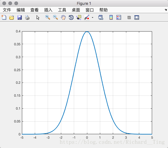
即:
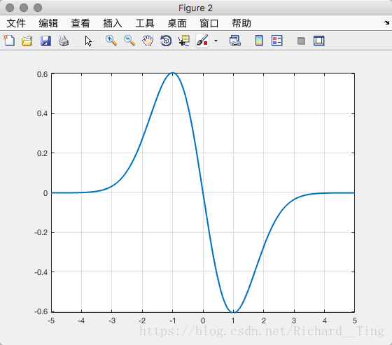
其中 , 为参数,我们去掉系数项,并且令 ,得到:
一阶求导后:
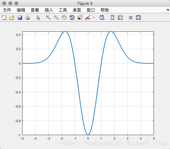
二阶求导后:
至此,我们告一段落,这些求导之后的结果将在明天给出实际用途。
Day4
- 1.2-D Gaussian Function
- 2.Using Gaussian Function to filter images
- 3.Scale Invariant
- 4.Object Orientation
- 5.Application
- Appendix
今天讲的内容还是很多de ~加油!
1. 2-D Gaussian Function
在讲二维Gaussian Function函数之前,让我们也回顾一下一维的。这些内容都挺重要的。
对了,还请一定复习一下之前的内容,因为知识点相关联。
1-D Gaussian function
(高斯公式-就是正态分布的公式)
其中
,
为参数,我们去掉系数项,并且令
,
一阶求导后:
二阶求导后:
2-D Gaussian function
现在让我们来学习一下二维Gaussian Function函数。
删繁就简,这里略去一切相关系数等知识,得到类似于1-D Gaussian function的2-D Gaussian function:
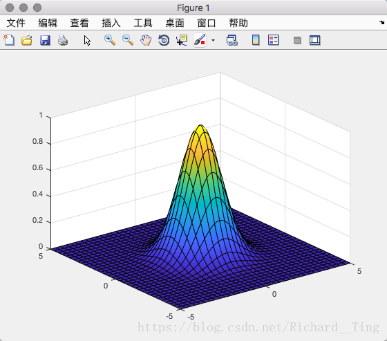
其一阶微分这里不再给出,主要讨论其对二阶LOG微分:
我们称其为 Laplacian of Gaussian (LOG)

这里的高斯函数,或者说正态分布是用来充当过滤器用的(见Day1中的 ,与其作用类似)
公式参考《概率论与数理统计教程》
参考1: 百度百科
参考2: https://www.cnblogs.com/pzxbc/archive/2012/02/14/2351708.html
参考3: https://blog.csdn.net/farmwang/article/details/78699926
参考4: https://www.cnblogs.com/herenzhiming/articles/5276106.html
2. Using Gaussian Function to filter images
看到这里,可能还是有人会疑惑,这个高斯函数究竟是做什么用的呢?
假设我们有一幅图像
,对其分别进行
与
变换。
即有
与
- 1.先考虑
,假设我们有以下图片
:
经过 处理后(即经过 ):

code:
>> I = rgb2gray(imread('Pentagram.jpg'));%灰度照片读取
>> imshow(I);%展示
>> out1=imgaussfilt(I,10);%sigma=10过滤
>> out2=imgaussfilt(I,20);%sigma=20过滤
>> figure;imshow(out1);
>> figure;imshow(out2);
结果为不同
取值的结果图:


So removes details from I, as is increased, larger details are removed.(所以这里的这个公式对原图像起到一个过滤的作用,除去noise,使得图像变模糊)
顺便欣赏一下这张图:

- 2.对于 ,其作用也有消去noise的,但是它的目的呢,是用来找图形对象的edge的,或者更准确地来讲,是来找图形object的size的。
为了能更好地理解这个高斯函数的作用,我们举出以下两个栗子。
1-D Gaussian function:一维例子

如上图,第一个序列是原始序列图
(就是这里的图片的像素点是1*n的);第二个序列图是经过原始 1-D Gaussian function (
) 处理过的,我们会发现,这个序列点的抖动性变弱,即noise变少;第三个序列图是经过 一阶 1-D Gaussian function (
) 变换得到的,请联系一下 Day2 的内容 —— 一阶求导最大值 —— 找到了edge的位置了;第四个序列图是经过 二阶 1-D Gaussian function (
) 变换得到的,请联系一下 Day2 的内容 —— 二阶求导取值为0 —— 同样找到了edge的位置了。

上面这幅图也是一个序列图,只不过其中还把 1-D Gaussian function 的图像画上了(如图橙色虚线部分)。这里需要讲解的是把上面六个序列图分为三组,每两个一组(一个变换前的序列图,一个变换后的序列图)。以第一组为例,变换前的序列图是指
和 二阶 1-D Gaussian function (
) 的图被画在第一个序列图中了,而
则被画在了第二个序列图中,同时它也是变换后的序列图。我们着重看最后一组图(第五个序列图和第六个序列图),(第五个序列图)我们发现序列图中蓝色部分取值为1的x范围和 二阶 1-D Gaussian function (
) 小于0的范围相同时,(第六个序列图)它们变换之后
的两个值构成的区间恰好为序列图中蓝色部分取值为1的x范围。由此得出结论,1-D Gaussian function 变换
是用来确定这个例子中序列的edge的(或者通俗地讲,确定序列不同取值的范围大小)。
2-D Gaussian function:二维例子
我们在一个白底中拟合出四个大小不同的点。

做了二维高斯变换
,得到下面四组图,而这里的作用更多的是确定点的size(大小)。

总结
1. 利用数学公式:
- 先看一维:
二阶求导是用来确定edge的位置的,从中恰好可以得到一个序列的区间。 - 再看二维:
二阶求导是用来确定edge的位置的,从中恰好可以得到一个图片object的size,有点类似圆。
2. 实际意义
- 总之,无论是一维,还是二维,只要这张图片不是 flat 的,我们就可以引入高斯函数(一般指的是二阶求导后的函数)进行过滤,同时不断调整 的取值加以过滤,过滤的过程同时就是找edge的过程,将满足edge的点连起来,在一维中就是一根线,在二维中就是一个面,也就是确定了一个图中object的大小,换句话说——detect the size of the object。
范例:
原始图像:

经过过滤:

调整
值

调整
值

调整
值

调整
值,最后得到一个较为满意的结果。

3. Scale Invariant
有了上面的高斯函数的解释后,就很容易解释缩放不变性了。无论我们的图片里需要确定的物体大小有多大,利用高斯函数都可以把它框出来,识别出来,这样就保证了缩放不变性啦!


4. Object Orientation
那么什么是Object Orientation呢?我们知道,一个能自动识别物体的无人驾驶的车一定要有足够快的技能去识别对面的物体,这就引出了一个问题,我们已经可以识别边了,那么如何快速识别?也就是在计算机识对象的时候,快速准确地确定边,这引申到数学问题中,相当于先要求一个函数值下降或上升最快的方向——梯度(gradient)。
那么具体是什么原理呢?
假设我们有一个白底黑块的图像
:(好吧,白底看的不清楚哈,哈哈~)

我们对
求一阶导(注意,这里的求导方式并非常规的,只是定义的一种求导方式,记作这样),并写成某种向量形式:
这里为什么不求二阶导数( )呢?因为求一阶导( )后仍是关于变量x与变量y的向量形式,我们知道,向量既有大小,又有方向,对我们后续求梯度方向有作用,而二阶导数( )不能做到这样。
于是,总结一下:
The direction of the gradient vector is given by
, the gradient vector points in the direction of max rate of the function.
有了这些原理后,就可以试着解决问题啦。
5. Application
这里图像识别的作用–查找,拼接