pytorch基础知识三

一.实现简单的全连接层

 1.权重和偏置自己构建

import torch as t
from torch import nn
#nn.Module能够利用autograd自动实现反向传播，这点比Function简单许多。
#调用layer(x)即可得到x对应的结果。
# 它等价于`layers.__call__(input)`，在`__call__`函数中，主要调用的是 `layer.forward(x)`
#在构造函数`__init__`中必须自己定义可学习的参数，并封装成`Parameter`，
# 如在本例中我们把`w`和`b`封装成`parameter`。`parameter`是一种特殊的`Tensor`，但其默认需要求导（requires_grad = True）
class Linear(nn.Module):  # 继承nn.Module
    def __init__(self, in_features, out_features):
        super(Linear, self).__init__()  # 等价于nn.Module.__init__(self)
        # nn.Module.__init__(self) 两种写法都可以 第一种推荐
        
        self.w = nn.Parameter(t.randn(in_features, out_features))
        self.b = nn.Parameter(t.randn(out_features))

    def forward(self, x):
        x = x.mm(self.w)  # x.@(self.w)
        return x + self.b.expand_as(x)

layer=Linear(4,3)
print(layer.w.shape)
x=t.rand(2,4)
for name, parameter in layer.named_parameters():
    print(name, parameter) # w and b

y=layer(x)
print(y.shape)

2.利用nn.linear实现

import torch as t
from torch import nn
# 输入 batch_size=2，维度3
x = t.randn(2, 4)
linear = nn.Linear(4, 3)
y = linear(x)
print(y.shape)
for name, parameter in nn.Linear.named_parameters(linear):
    print(name, parameter) # w and b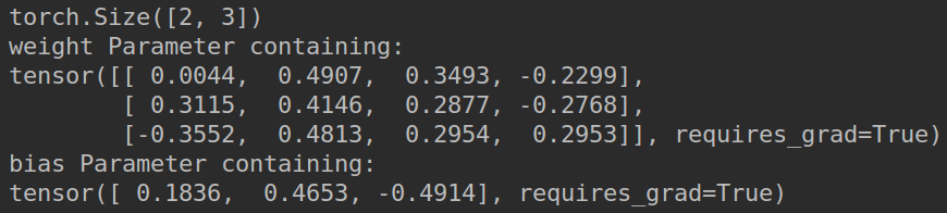

二,实现卷积

1.Sequential的三种实现方式

#在以上的例子中，基本上都是将每一层的输出直接作为下一层的输入，这种网络称为前馈传播网络（feedforward neural network）
#。对于此类网络如果每次都写复杂的forward函数会有些麻烦，在此就有两种简化方式，
#ModuleList和Sequential。其中Sequential是一个特殊的module，它包含几个子Module，
#前向传播时会将输入一层接一层的传递下去。ModuleList也是一个特殊的module，
#可以包含几个子module，可以像用list一样使用它，但不能直接把输入传给ModuleList
from torch import nn
import torch as t
# Sequential的三种写法
#FIRST
net1 = nn.Sequential()
net1.add_module('conv', nn.Conv2d(3, 3, 3))
net1.add_module('batchnorm', nn.BatchNorm2d(3))
net1.add_module('activation_layer', nn.ReLU())
print('net1:', net1)
#SECOND
net2 = nn.Sequential(
        nn.Conv2d(3, 3, 3),
        nn.BatchNorm2d(3),
        nn.ReLU()
        )
print('net2:', net2)

#THIRD
from collections import OrderedDict
net3= nn.Sequential(OrderedDict([
          ('conv1', nn.Conv2d(3, 3, 3)),
          ('bn1', nn.BatchNorm2d(3)),
          ('relu1', nn.ReLU())
        ]))
print('net3:', net3)

x = t.rand(1, 3, 4, 4)
output = net1(x)
print(output.shape)
output = net2(x)
print(output.shape)
output = net3(x)
print(output.shape)

2.ModuleList

#Modelu list 实现
modellist = nn.ModuleList([nn.Conv2d(3, 3, 3), nn.BatchNorm2d(3), nn.ReLU()])
x = t.randn(1, 3,4,4)
for model in modellist:
    print(model)

三,实现逻辑回归

import torch
import matplotlib.pyplot as plt
from torch import nn,optim
from torch.autograd import Variable

import numpy as np

def produce_data():
    # 假数据
    n_data = torch.ones(100, 2)  # 数据的基本形态
    x0 = torch.normal(2 * n_data, 1)  # 类型0 x data (tensor), shape=(100, 2)
    y0 = torch.zeros(100)  # 类型0 y data (tensor), shape=(100, 1)
    x1 = torch.normal(-2 * n_data, 1)  # 类型1 x data (tensor), shape=(100, 1)
    y1 = torch.ones(100)  # 类型1 y data (tensor), shape=(100, 1)
    print(x0.shape)
    # 注意 x, y 数据的数据形式是一定要像下面一样 (torch.cat 是在合并数据)
    x = torch.cat((x0, x1), 0).type(torch.FloatTensor)  # FloatTensor = 32-bit floating
    print(x.shape)
    y = torch.cat((y0, y1), 0).type(torch.FloatTensor)  # LongTensor = 64-bit integer
    print(y.shape)
    # 画图
    # plt.scatter(x.data.numpy()[:, 0], x.data.numpy()[:, 1], c=y.data.numpy(), s=100, lw=0, cmap='RdYlGn')
    # plt.show()
    return x,y


class LogisticRegression(nn.Module):
    def __init__(self):
        super(LogisticRegression,self).__init__()
        self.lr=nn.Linear(2,1)
        self.s=nn.Sigmoid()

    def forward(self,x):
        x=self.lr(x)
        x=self.s(x)
        return x


if __name__ == '__main__':
    x,y=produce_data()
    lr_model=LogisticRegression()
    if torch.cuda.is_available():
        lr_model.cuda()
    criterion=nn.BCELoss()
    optimizer=optim.Adam(lr_model.parameters(),lr=1e-3)

    plt.figure()
    for epoch in range(1000):
        if torch.cuda.is_available():
            x_data = Variable(x).cuda()
            y_data = Variable(y).cuda()
        else:
            x_data = Variable(x)
            y_data = Variable(y)

        y_pred=lr_model(x_data)
        loss=criterion(y_pred,y_data)
        print_loss=loss.item()
        # print(print_loss)
        #compute acc
        mask = y_pred.ge(0.5).float()  # 以0.5为阈值进行分类
        # print(len(mask))
        correct=(mask==y_data).sum()
        acc = correct.item() / x_data.size(0)  # 计算精度
        optimizer.zero_grad()
        loss.backward()
        optimizer.step()

        # 每隔20轮打印一下当前的误差和精度
        if (epoch + 1) % 20 == 0:
            print('*' * 10)
            print('epoch {}'.format(epoch + 1))  # 训练轮数
            print('loss is {:.4f}'.format(print_loss))  # 误差
            print('acc is {:.4f}'.format(acc))



    # 结果可视化
    #x0*w0+y0*w1+b=0
    w0, w1 = lr_model.lr.weight[0]
    print(lr_model.lr.weight)
    w0 = float(w0.item())
    w1 = float(w1.item())
    b = float(lr_model.lr.bias.item())
    plot_x = np.arange(-4, 4, 0.1)
    plot_y = -(w0 * plot_x + b) / w1
    plt.scatter(x.data.numpy()[:, 0], x.data.numpy()[:, 1], c=y.data.numpy(), s=100, lw=0, cmap='RdYlGn')
    plt.plot(plot_x, plot_y)

    plt.show()