pytorch1.0实现AutoEncoder

AutoEncoder (自编码器-非监督学习)
神经网络也能进行非监督学习, 只需要训练数据, 不需要标签数据. 自编码就是这样一种形式.
自编码能自动分类数据, 而且也能嵌套在半监督学习的上面, 用少量的有标签样本和大量的无标签样本学习.

import torch
import torch.nn as nn
import torch.utils.data as Data
import torchvision
import matplotlib.pyplot as plt
from mpl_toolkits.mplot3d import Axes3D
from matplotlib import cm
import numpy as np

# 超参数
# Hyper Parameters
EPOCH = 10
BATCH_SIZE = 64
LR = 0.005            # learning rate
DOWNLOAD_MNIST = True # False   # 下过数据的话,可以设置成 False
N_TEST_IMG = 5        # 到时候显示5张图片看效果

# 下载数据
# Mnist digits dataset
train_data = torchvision.datasets.MNIST(
    root='./mnist/',
    train=True,                                     # this is training data
    transform=torchvision.transforms.ToTensor(),    # Converts a PIL.Image or numpy.ndarray to
                                                    # torch.FloatTensor of shape (C x H x W) and normalize in the range [0.0, 1.0]
    download=DOWNLOAD_MNIST,                        # download it if you don't have it
)

# plot one example
print(train_data.train_data.size())     # (60000, 28, 28)
print(train_data.train_labels.size())   # (60000)
plt.imshow(train_data.train_data[2].numpy(), cmap='gray')
plt.title('%i' % train_data.train_labels[2])
plt.show()

# 加载训练数据
# Data Loader for easy mini-batch return in training, the image batch shape will be (50, 1, 28, 28)
train_loader = Data.DataLoader(dataset=train_data, batch_size=BATCH_SIZE, shuffle=True)

# AutoEncoder
# AutoEncoder 形式很简单, 分别是 encoder 和 decoder, 压缩和解压, 压缩后得到压缩的特征值, 再从压缩的特征值解压成原图片.
class AutoEncoder(nn.Module):
    def __init__(self):
        super(AutoEncoder, self).__init__()
        # 压缩
        self.encoder = nn.Sequential(
            nn.Linear(28*28, 128),
            nn.Tanh(),
            nn.Linear(128, 64),
            nn.Tanh(),
            nn.Linear(64, 12),
            nn.Tanh(),
            nn.Linear(12, 3),   # compress to 3 features which can be visualized in plt # 压缩成3个特征, 进行 3D 图像可视化
        )
        # 解压
        self.decoder = nn.Sequential(
            nn.Linear(3, 12),
            nn.Tanh(),
            nn.Linear(12, 64),
            nn.Tanh(),
            nn.Linear(64, 128),
            nn.Tanh(),
            nn.Linear(128, 28*28),
            nn.Sigmoid(),       # compress to a range (0, 1) # 激励函数让输出值在 (0, 1)
        )
    def forward(self, x):
        encoded = self.encoder(x)
        decoded = self.decoder(encoded)
        return encoded, decoded

autoencoder = AutoEncoder()

optimizer = torch.optim.Adam(autoencoder.parameters(), lr=LR)
loss_func = nn.MSELoss()

# initialize figure
f, a = plt.subplots(2, N_TEST_IMG, figsize=(5, 2))
plt.ion()   # continuously plot

# original data (first row) for viewing
view_data = train_data.train_data[:N_TEST_IMG].view(-1, 28*28).type(torch.FloatTensor)/255.
for i in range(N_TEST_IMG):
    a[0][i].imshow(np.reshape(view_data.data.numpy()[i], (28, 28)), cmap='gray'); a[0][i].set_xticks(()); a[0][i].set_yticks(())

# 训练
# 可以有效的利用 encoder 和 decoder 来做很多事, 比如这里我们用 decoder 的信息输出看和原图片的对比,
# 还能用 encoder 来看经过压缩后, 神经网络对原图片的理解. encoder 能将不同图片数据大概的分离开来.
# 这样就是一个无监督学习的过程.
for epoch in range(EPOCH):
    for step, (x, b_label) in enumerate(train_loader):
        b_x = x.view(-1, 28*28)   # batch x, shape (batch, 28*28)
        b_y = x.view(-1, 28*28)   # batch y, shape (batch, 28*28)

        encoded, decoded = autoencoder(b_x)

        loss = loss_func(decoded, b_y)      # mean square error
        optimizer.zero_grad()               # clear gradients for this training step
        loss.backward()                     # backpropagation, compute gradients
        optimizer.step()                    # apply gradients

        if step % 100 == 0:
            print('Epoch: ', epoch, '| train loss: %.4f' % loss.data.numpy())

            # plotting decoded image (second row)
            _, decoded_data = autoencoder(view_data)
            for i in range(N_TEST_IMG):
                a[1][i].clear()
                a[1][i].imshow(np.reshape(decoded_data.data.numpy()[i], (28, 28)), cmap='gray')
                a[1][i].set_xticks(()); a[1][i].set_yticks(())
            plt.draw(); plt.pause(0.05)

plt.ioff()
plt.show()

# 画3D图
# visualize in 3D plot
# 要观看的数据
view_data = train_data.train_data[:200].view(-1, 28*28).type(torch.FloatTensor)/255.
encoded_data, _ = autoencoder(view_data)  # 提取压缩的特征值
fig = plt.figure(2)
ax = Axes3D(fig)  # 3D 图
# x, y, z 的数据值
X, Y, Z = encoded_data.data[:, 0].numpy(), encoded_data.data[:, 1].numpy(), encoded_data.data[:, 2].numpy()
values = train_data.train_labels[:200].numpy()   # 标签值
for x, y, z, s in zip(X, Y, Z, values):
    c = cm.rainbow(int(255*s/9))             # 上色
    ax.text(x, y, z, s, backgroundcolor=c)   # 标位子
ax.set_xlim(X.min(), X.max()); ax.set_ylim(Y.min(), Y.max()); ax.set_zlim(Z.min(), Z.max())
plt.show()

有时神经网络要接受大量的输入信息, 比如输入信息是高清图片时, 输入信息量可能达到上千万, 让神经网络直接从上千万个信息源中学习是一件很吃力的工作.

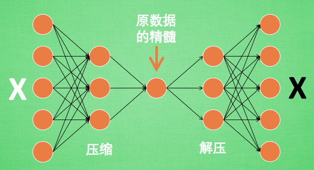
所以, 何不压缩一下, 提取出原图片中的最具代表性的信息, 缩减输入信息量, 再把缩减过后的信息放进神经网络学习. 这样学习起来就简单轻松了.

所以, 自编码就能在这时发挥作用. 通过将原数据白色的X 压缩, 解压成黑色的X, 然后通过对比黑白 X ,求出预测误差, 进行反向传递, 逐步提升自编码的准确性.

训练好的自编码中间这一部分就是能总结原数据的精髓. 可以看出, 从头到尾, 我们只用到了输入数据 X, 并没有用到 X 对应的数据标签, 所以也可以说自编码是一种非监督学习.

到了真正使用自编码的时候. 通常只会用到自编码前半部分.

pytorch1.0实现AutoEncoder

猜你喜欢