opencv-python-学习笔记十（图像阈值）

简单阈值

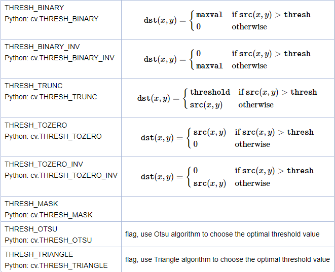
对每一个像素都应用相同的阈值。如果像素值小于阈值，则将其设置为0，否则设置为最大值。cv.threshold函数用于设置阈值，它的第一个参数是源图像的灰度图像，第二个参数是用于对像素值进行分类的阈值，第三个参数是分配给超过阈值的像素值的最大值。OpenCV提供了不同类型的阈值，阈值类型由函数的第四个参数给出。

函数：

retval, dst=cv.threshold(src, thresh, maxval, type[, dst])对每个像素使用固定的阈值

参数：

src	输入图像 ，灰度图(多通道, 8-bit or 32-bit floating point).
dst	与src具有相同大小、类型和通道数的输出数组。
thresh	阈值
maxval	当像素值超过了阈值（或者小于阈值，根据type来决定），所赋予的值
type	阈值类型 (see ThresholdTypes).

返回值：

 retVal：使用的阈值，在Otsu‘s中会用到

 dst： 经过阈值处理的图像

阈值类型：

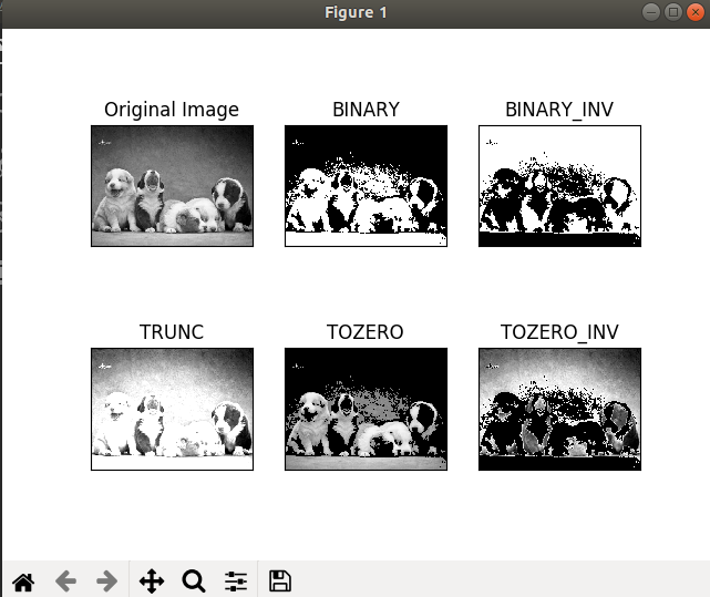
举例：

import cv2 as cv
import numpy as np
from matplotlib import pyplot as plt
img = cv.imread('4.jpg', 0)
ret, thresh1 = cv.threshold(img, 127, 255, cv.THRESH_BINARY)
ret, thresh2 = cv.threshold(img, 127, 255, cv.THRESH_BINARY_INV)
ret, thresh3 = cv.threshold(img, 127, 255, cv.THRESH_TRUNC)
ret, thresh4 = cv.threshold(img, 127, 255, cv.THRESH_TOZERO)
ret, thresh5 = cv.threshold(img, 127, 255, cv.THRESH_TOZERO_INV)
titles = ['Original Image', 'BINARY',
          'BINARY_INV', 'TRUNC', 'TOZERO', 'TOZERO_INV']
images = [img, thresh1, thresh2, thresh3, thresh4, thresh5]
for i in range(6):
    plt.subplot(2, 3, i+1), plt.imshow(images[i], 'gray')
    plt.title(titles[i])
    plt.xticks([]), plt.yticks([])
plt.show()

 

自适应阈值

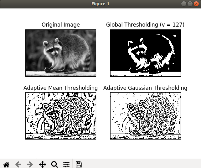
在上一节中，我们使用一个全局值作为阈值。但这并不适用于所有情况，例如，如果一张图像在不同的区域有不同的光照条件。在这种情况下，自适应阈值阈值可以提供帮助，算法会根据像素周围的小区域来确定像素的阈值。因此，对于同一幅图像的不同区域，我们得到了不同的阈值，对于光照不同的图像，我们得到了更好的结果。除了上述所描述的区域外，cv.adaptiveThreshold函数还需要3个其它参数。

函数

dst=cv.adaptiveThreshold(src, maxValue, adaptiveMethod, thresholdType, blockSize, C[, dst])

参数：

src	源 8-bit 单通道图像
dst	与源图像具有相同大小和类型的目标图像
maxValue	当像素值超过了阈值（或者小于阈值，根据type来决定），所赋予的值
adaptiveMethod	阈值的计算方法，包含以下2种类型： see AdaptiveThresholdTypes.
thresholdType	阈值类型必须是 THRESH_BINARY or THRESH_BINARY_INV
blockSize	像素邻域的大小，用来计算像素的阈值: 3, 5, 7, and so on.
C	阈值计算方法中的常数项

上述参数中，adaptiveMethod决定了阈值是如何计算的

　　cv.ADAPTIVE_THRESH_MEAN_C： 阈值是邻域面积减去常数C的平均值。

　　cv2.ADAPTIVE_THRESH_GAUSSIAN_C：阈值是邻域值减去常数C的高斯加权和，权重为一个高斯窗口

blockSize大小决定了邻域的大小，C是从邻域像素的均值或加权和中减去的常数。

举例

import cv2 as cv
import numpy as np
from matplotlib import pyplot as plt
img = cv.imread('2.png',0)
# 中值滤波，抑制图像噪声。在滤除噪声的同时，能够保护信号的边缘，使之不被模糊
img = cv.medianBlur(img,5)
# 简单阈值
ret,th1 = cv.threshold(img,127,255,cv.THRESH_BINARY)
# 自适应阈值
th2 = cv.adaptiveThreshold(img,255,cv.ADAPTIVE_THRESH_MEAN_C,\
            cv.THRESH_BINARY,11,2)
th3 = cv.adaptiveThreshold(img,255,cv.ADAPTIVE_THRESH_GAUSSIAN_C,\
            cv.THRESH_BINARY,11,2)
titles = ['Original Image', 'Global Thresholding (v = 127)',
            'Adaptive Mean Thresholding', 'Adaptive Gaussian Thresholding']
images = [img, th1, th2, th3]
for i in range(4):
    plt.subplot(2,2,i+1),plt.imshow(images[i],'gray')
    plt.title(titles[i])
    plt.xticks([]),plt.yticks([])
plt.show()

Otsu's二值化

在全局阈值化中，我们使用一个任意选择的值作为阈值。相反，Otsu的方法避免了必须选择一个值并自动确定它。

Otsu’s Binarization是一种基于直方图的二值化方法，它需要和threshold函数配合使用。

考虑只有两个不同图像值的图像(双峰图像)，其中直方图只包含两个峰值。一个好的阈值应该位于这两个值的中间（对于非双峰图像，这种方法 得到的结果可能会不理想）。同样，Otsu的方法从图像直方图中确定一个最优的全局阈值。

为此，使用 cv.threshold()函数， cv.THRESH_OTSU 最为一个额外的标志传入。阈值可以任意选择。然后，该算法找找出一个最优阈值最为第一个输出。

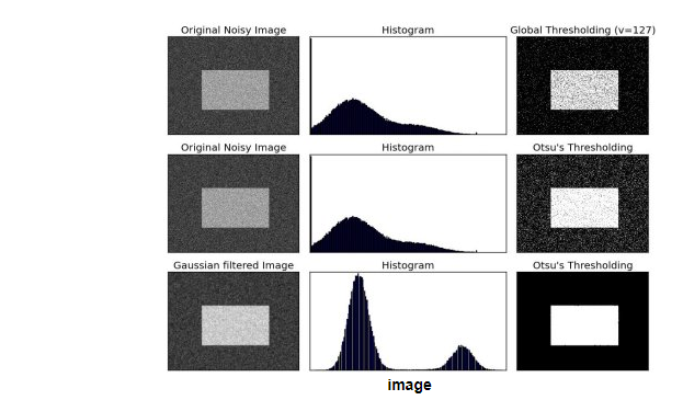
看一下下边的例子。输入图像是一个有噪声的图像，在第一种情况下，应用值为127的全局阈值。在第二种情况下，直接应用Otsu的阈值。在第三种情况下，首先用5x5高斯核对图像进行滤波，去除噪声，然后应用Otsu阈值。看看噪声滤波如何改进结果。

import cv2 as cv
import numpy as np
from matplotlib import pyplot as plt
img = cv.imread('noisy2.png',0)
# global thresholding
ret1,th1 = cv.threshold(img,127,255,cv.THRESH_BINARY)
# Otsu's thresholding
ret2,th2 = cv.threshold(img,0,255,cv.THRESH_BINARY+cv.THRESH_OTSU)
# Otsu's thresholding after Gaussian filtering
blur = cv.GaussianBlur(img,(5,5),0)
# 阈值一定要设为0
ret3,th3 = cv.threshold(blur,0,255,cv.THRESH_BINARY+cv.THRESH_OTSU)
# plot all the images and their histograms
images = [img, 0, th1,
          img, 0, th2,
          blur, 0, th3]
titles = ['Original Noisy Image','Histogram','Global Thresholding (v=127)',
          'Original Noisy Image','Histogram',"Otsu's Thresholding",
          'Gaussian filtered Image','Histogram',"Otsu's Thresholding"]
for i in xrange(3):
    plt.subplot(3,3,i*3+1),plt.imshow(images[i*3],'gray')
    plt.title(titles[i*3]), plt.xticks([]), plt.yticks([])
    plt.subplot(3,3,i*3+2),plt.hist(images[i*3].ravel(),256)
    plt.title(titles[i*3+1]), plt.xticks([]), plt.yticks([])
    plt.subplot(3,3,i*3+3),plt.imshow(images[i*3+2],'gray')
    plt.title(titles[i*3+2]), plt.xticks([]), plt.yticks([])
plt.show()

Otsu过程： 
1. 计算图像直方图； 
2. 设定一阈值，把直方图强度大于阈值的像素分成一组，把小于阈值的像素分成另外一组； 
3. 分别计算两组内的偏移数，并把偏移数相加； 
4. 把0~255依照顺序多为阈值，重复1-3的步骤，直到得到最小偏移数，其所对应的值即为结果阈值。