背景
上一篇文章介绍了FNN [2],在FM的基础上引入了DNN对特征进行高阶组合提高模型表现。但FNN并不是完美的,针对FNN的缺点上交与UCL于2016年联合提出一种新的改进模型PNN(Product-based Neural Network)。
PNN同样引入了DNN对低阶特征进行组合,但与FNN不同,PNN并没有单纯使用全连接层来对低阶特征进行组合,而是设计了Product层对特征进行更细致的交叉运算。在《推荐系统系列(三):FNN理论与实践》中提到过,在不考虑激活函数的前提下,使用全连接的方式对特征进行组合,等价于将所有特征进行加权求和。PNN的作者同样意识到了这个问题,认为“加法”操作并不足以捕获不同Field特征之间的相关性。原文如下 [1]:
the “add” operations of the perceptron layer might not be useful to explore the interactions of categorical data in multiple fields.
有研究表明“product”操作比“add”操作更有效,而且FM模型的优势正是通过特征向量的内积来体现的。基于此,PNN作者设计了product layer来对特征进行组合,包含内积与外积两种操作。实验表明,PNN有显著提升,而product layer也成为了深度推荐模型中的经典结构。
分析
1. PNN结构
PNN的网络架构如下图所示:

从上往下进行分析,最上层输出的是预估的CTR值,\(\hat{y}=\sigma(W_3l_2+b_3)\) ,公式符号与原Paper保持一致。
第二层隐藏层:\(l_2=relu(W_2l_1+b_1)\)
第一层隐藏层:$l_1=relu(l_z+l_p+b_1) $
PNN核心在于计算 \(l_z,l_p\) 。首先,定义矩阵点积运算 \(A \bigodot B \triangleq \sum_{i,j}A_{i,j}B_{i,j}\)
则:
\[ \begin{align} l_z=(l_{z}^1,l_{z}^2,\dots,l_{z}^n,\dots,l_{z}^{D_1}), \qquad l_z^n=W_z^n \bigodot z \notag \\ \end{align} \tag{1} \]
\[ \begin{align} l_p=(l_{p}^1,l_{p}^2,\dots,l_{p}^n,\dots,l_{p}^{D_1}), \qquad l_p^n=W_p^n \bigodot p \notag \\ \end{align} \tag{2} \]
其中:
\[ \begin{align} z=(z_1,z_2,\dots,z_N) \triangleq (f_1,f_2,\dots,f_N) \notag \\ \end{align} \tag{3} \]
\[ \begin{align} p=\{p_{i,j}\},i=1 \dots N,j=1 \dots N \notag \\ \end{align} \tag{4} \]
结合公式(1)(3),得:
\[ \begin{align} l_z^n=W_z^n \bigodot z=\sum_{i=1}^N\sum_{j=1}^M(W_z^n)_{i,j}z_{i,j} \notag \\ \end{align} \tag{5} \]
公式(3)中,\(f_i \in \mathbb{R}^M\) 表示经过embedding之后的特征向量,embedding过程与FNN保持一致。联系PNN结构图与公式(1)(3)可以看出,这个部分的计算主要是为了保留低阶特征,对比FNN丢弃低阶特征,只对二阶特征进行更高阶组合,显然PNN是为了弥补这个缺点。
公式(4)中 \(p_{i,j}=g(f_i,f_j)\) 表示成对特征交叉函数,定义不同的交叉方式也就有不同的PNN结构。在论文中,函数 \(g(f_i,f_j)\) 有两种表示,第一种为向量内积运算,即IPNN(Inner Product-based Neural Network);第二种为向量外积运算,即OPNN(Outer Product-based Neural Network)。
1.1 IPNN分析
定义 \(p_{i,j}=g(f_i,f_j)=\langle f_i,f_j \rangle\) ,将公式(2)进行改写,得:
\[ \begin{align} l_p^n=W_p^n \bigodot p=\sum_{i=1}^N\sum_{j=1}^N(W_p^n)_{i,j}p_{i,j}= \sum_{i=1}^N\sum_{j=1}^N(W_p^n)_{i,j}\langle f_i,f_j \rangle \notag \\ \end{align} \tag{6} \]
分析IPNN的product layer计算空间复杂度:
结合公式(1)(5)可知,\(l_z\) 计算空间复杂度为 \(O(D_1NM)\) 。结合公式(2)(6)可知,计算 \(p\) 需要 \(O(N^2)\) 空间开销,\(l_p^n\) 需要 \(O(N^2)\) 空间开销,所以 \(l_p\) 计算空间复杂度为 \(O(D_1NN)\) 。所以,product layer 整体计算空间复杂度为 \(O(D_1N(M+N))\) 。
分析IPNN的product layer计算时间复杂度:
结合公式(1)(5)可知,\(l_z\) 计算时间复杂度为 \(O(D_1NM)\) 。结合公式(2)(6)可知,计算 \(p_{i,j}\) 需要 \(O(M)\) 时间开销,计算 \(p\) 需要 \(O(N^2M)\) 时间开销,又因为 \(l_p^n\) 需要 \(O(N^2)\) 时间开销,所以 \(l_p\) 计算空间复杂度为 \(O(N^2(M+D_1))\) 。所以,product layer 整体计算时间复杂度为 \(O(N^2(M+D_1))\) 。
计算优化
时空复杂度过高不适合工程实践,所以需要进行计算优化。因为 \(l_z\) 本身计算开销不大,所以将重点在于优化 \(l_p\) 的计算,更准确一点在于优化公式(6)的计算。
受FM的参数矩阵分解启发,由于 \(p_{i,j},W_p^n\) 都是对称方阵,所以使用一阶矩阵分解,假设 \(W_p^n=\theta^n\theta^{nT}\) ,此时有 \(\theta^n \in \mathbb{R}^N\) 。将原本参数量为 \(N*N\) 的矩阵 \(W_p^n\) ,分解为了参数量为 \(N\) 的向量 \(\theta^n\) 。同时,将公式(6)改写为:
\[ \begin{align} l_p^n ={} & W_p^n \bigodot p =\sum_{i=1}^N\sum_{j=1}^N(W_p^n)_{i,j}\langle f_i,f_j \rangle \notag \\ ={} & \sum_{i=1}^N\sum_{j=1}^N \theta_i^n \theta_j^n \langle f_i,f_j \rangle \notag \\ ={} &\sum_{i=1}^N\sum_{j=1}^N \langle \theta_i^nf_i, \theta_j^nf_j \rangle \notag \\ ={} & \langle \sum_{i=1}^N\theta_i^nf_i, \sum_{j=1}^N\theta_j^nf_j \rangle \notag \\ ={} & \langle \sum_{i=1}^N\delta_i^n, \sum_{j=1}^N\delta_j^n \rangle \notag \\ ={} & \Vert \sum_{i=1}^N\delta_i^n \Vert^2 \notag \\ \end{align} \tag{7} \]
其中:\(\delta_i^n=\theta_i^nf_i\) ,\(\delta_i^n \in \mathbb{R}^M\) 。结合公式(2)(7),得:
\[ \begin{align} l_p=(\Vert \sum_{i=1}^N\delta_i^1 \Vert^2,\dots,\Vert \sum_{i=1}^N\delta_i^n \Vert^2,\dots,\Vert \sum_{i=1}^N\delta_i^{D_1} \Vert^2) \notag \\ \end{align} \tag{8} \]
优化后的时空复杂度
空间复杂度由\(O(D_1N(M+N))\) 降为 \(O(D_1NM)\) ;
时间复杂度由\(O(N^2(M+D_1))\) 降为 \(O(D_1NM)\) ;
虽然通过参数矩阵分解可以对计算开销进行优化,但由于采用一阶矩阵分解来近似矩阵结果,所以会丢失一定的精确性。如果考虑引入K阶矩阵分解,虽然精度更高但计算开销会更高。
1.2 OPNN分析
将特征交叉的方式由内积变为外积,便可以得到PNN的另一种形式OPNN。
定义 \(p_{i,j}=g(f_i,f_j)=f_if_j^T\) ,将公式(2)进行改写,得到:
\[ \begin{align} l_p^n=W_p^n \bigodot p=\sum_{i=1}^N\sum_{j=1}^N(W_p^n)_{i,j}p_{i,j}= \sum_{i=1}^N\sum_{j=1}^N(W_p^n)_{i,j}f_if_j^T \notag \\ \end{align} \tag{9} \]
类似于IPNN的分析,OPNN的时空复杂度均为 \(O(D_1M^2N^2)\) 。
为了进行计算优化,引入叠加的概念(sum pooling)。将 \(p\) 的计算公式重新定义为:
\[ \begin{align} p=\sum_{i=1}^N\sum_{j=1}^Nf_if_j^T=f_{\sum}f_{\sum}^T, \qquad f_{\sum}=\sum_{i=1}^Nf_i \notag \\ \end{align} \tag{10} \]
那么公式(9)重新定义为:(注意,此时 \(p \in \mathbb{R}^{M \times M}\) )
\[ \begin{align} l_p^n=W_p^n \bigodot p=\sum_{i=1}^M\sum_{j=1}^M(W_p^n)_{i,j}p_{i,j} \notag \\ \end{align} \tag{11} \]
通过公式(10)可知, \(f_{\sum}\) 的时间复杂度为 \(O(MN)\) ,\(p\) 的时空复杂度均为 \(O(MM)\) , \(l_p^n\) 的时空复杂度均为 \(O(MM)\) ,那么计算 \(l_p\) 的时空复杂度均为 \(O(D_1MM)\) ,从上一小节可知,计算 \(l_z\) 的时空复杂度均为 \(O(D_1MN)\) 。所以最终OPNN的时空复杂度为 \(O(D_1M(M+N))\) 。
那么OPNN的时空复杂度由 \(O(D_1M^2N^2)\) 降低到 \(O(D_1M(M+N))\) 。
同样的,虽然叠加概念的引入可以降低计算开销,但是中间的精度损失也是很大的,性能与精度之间的tradeoff。
降低复杂度的具体策略与具体的product函数选择有关,IPNN其实通过矩阵分解,“跳过”了显式的product层,通过代数转换直接从embedding层一步到位到 \(l_1\) 隐层,而OPNN则是直接在product层入手进行优化 [3]
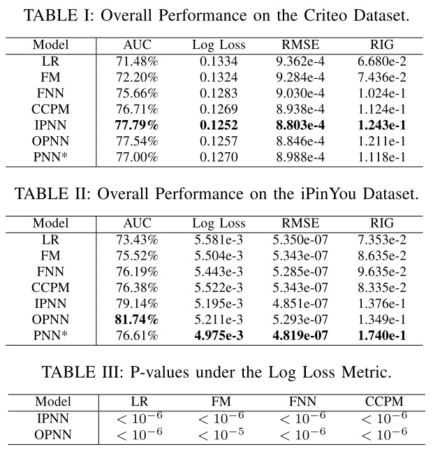
2. 性能分析
作者在 \(Criteo\) 与 \(iPinYou\) 数据集上进行实验,对比结果如下。其中 \(PNN^*\) 是同时对特征进行内积与外积计算,然后concat在一起送入下一层。

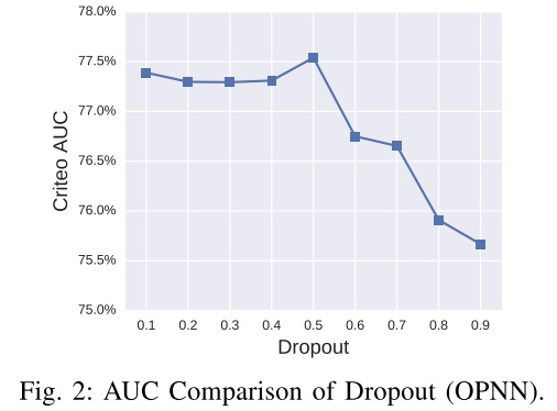
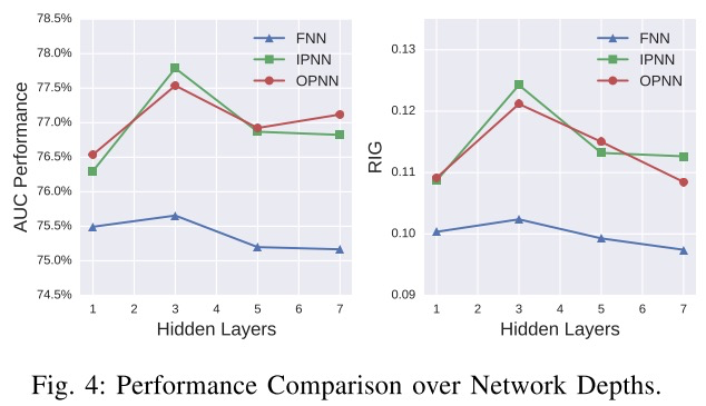
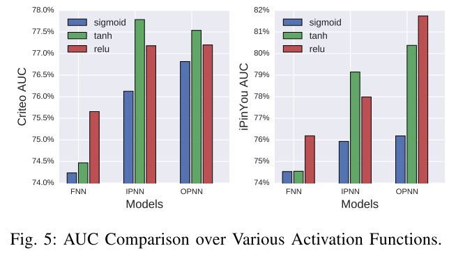
关于模型dropout比例、激活函数以及隐藏层参数的实验对比如下所示:
3. 优缺点
优点:
- 对比FNN,在进行高阶特征组合的同时,融入了低阶特征,且无需进行两阶段训练。
实验
使用 \(MovieLens100K dataset\) ,核心代码如下。
class PNN(object):
    def __init__(self, vec_dim=None, field_lens=None, lr=None, dnn_layers=None, dropout_rate=None, lamda=None, use_inner=True):
        self.vec_dim = vec_dim
        self.field_lens = field_lens
        self.field_num = len(field_lens)
        self.lr = lr
        self.dnn_layers = dnn_layers
        self.dropout_rate = dropout_rate
        self.lamda = float(lamda)
        self.use_inner = use_inner
        assert dnn_layers[-1] == 1
        self.l2_reg = tf.contrib.layers.l2_regularizer(self.lamda)

        self._build_graph()

    def _build_graph(self):
        self.add_input()
        self.inference()

    def add_input(self):
        self.x = [tf.placeholder(tf.float32, name='input_x_%d'%i) for i in range(self.field_num)]
        self.y = tf.placeholder(tf.float32, shape=[None], name='input_y')
        self.is_train = tf.placeholder(tf.bool)

    def inference(self):
        with tf.variable_scope('emb_part'):
            emb = [tf.get_variable(name='emb_%d'%i, shape=[self.field_lens[i], self.vec_dim], dtype=tf.float32, regularizer=self.l2_reg) for i in range(self.field_num)]
            emb_layer = tf.concat([tf.matmul(self.x[i], emb[i]) for i in range(self.field_num)], axis=1) # (batch, F*K)
            emb_layer = tf.reshape(emb_layer, shape=[-1, self.field_num, self.vec_dim]) # (batch, F, K)

        with tf.variable_scope('linear_part'):
            linear_part = tf.reshape(emb_layer, shape=[-1, self.field_num*self.vec_dim]) # (batch, F*K)
            linear_w = tf.get_variable(name='linear_w', shape=[self.field_num*self.vec_dim, self.dnn_layers[0]], dtype=tf.float32, regularizer=self.l2_reg) # (F*K, D)
            self.lz = tf.matmul(linear_part, linear_w) # (batch, D)

        with tf.variable_scope('product_part'):
            product_out = []
            if self.use_inner:
                inner_product_w = tf.get_variable(name='inner_product_w', shape=[self.dnn_layers[0], self.field_num], dtype=tf.float32, regularizer=self.l2_reg) # (D, F)
                for i in range(self.dnn_layers[0]):
                    delta = tf.multiply(emb_layer, tf.expand_dims(inner_product_w[i], axis=1)) # (batch, F, K)
                    delta = tf.reduce_sum(delta, axis=1) # (batch, K)
                    product_out.append(tf.reduce_sum(tf.square(delta), axis=1, keep_dims=True)) # (batch, 1)
            else:
                outer_product_w = tf.get_variable(name='outer_product_w', shape=[self.dnn_layers[0], self.vec_dim, self.vec_dim], dtype=tf.float32, regularizer=self.l2_reg) # (D, K, K)
                field_sum = tf.reduce_sum(emb_layer, axis=1) # (batch, K)
                p = tf.matmul(tf.expand_dims(field_sum, axis=2), tf.expand_dims(field_sum, axis=1)) # (batch, K, K)
                for i in range(self.dnn_layers[0]):
                    lpi = tf.multiply(p, tf.expand_dims(outer_product_w[i], axis=0)) # (batch, K, K)
                    product_out.append(tf.expand_dims(tf.reduce_sum(lpi, axis=[1,2]), axis=1)) # (batch, 1)
            self.lp = tf.concat(product_out, axis=1)  # (batch, D)
            bias = tf.get_variable(name='bias', shape=[self.dnn_layers[0]], dtype=tf.float32)
            self.product_layer = tf.nn.relu(self.lz+self.lp+bias)

        x = self.product_layer
        in_node = self.dnn_layers[0]
        with tf.variable_scope('dnn_part'):
            for i in range(1, len(self.dnn_layers)):
                out_node = self.dnn_layers[i]
                w = tf.get_variable(name='w_%d'%i, shape=[in_node, out_node], dtype=tf.float32, regularizer=self.l2_reg)
                b = tf.get_variable(name='b_%d'%i, shape=[out_node], dtype=tf.float32)
                x = tf.matmul(x, w) + b
                if out_node == 1:
                    self.y_logits = x
                else:
                    x = tf.layers.dropout(tf.nn.relu(x), rate=self.dropout_rate, training=self.is_train)
                in_node = out_node

        self.y_hat = tf.nn.sigmoid(self.y_logits)
        self.pred_label = tf.cast(self.y_hat > 0.5, tf.int32)
        self.loss = -tf.reduce_mean(self.y*tf.log(self.y_hat+1e-8) + (1-self.y)*tf.log(1-self.y_hat+1e-8))
        reg_variables = tf.get_collection(tf.GraphKeys.REGULARIZATION_LOSSES)
        if len(reg_variables) > 0:
            self.loss += tf.add_n(reg_variables)
        self.train_op = tf.train.AdamOptimizer(self.lr).minimize(self.loss)
reference
[1] Qu, Yanru, et al. "Product-based neural networks for user response prediction." 2016 IEEE 16th International Conference on Data Mining (ICDM). IEEE, 2016.
[2] Zhang, Weinan, Tianming Du, and Jun Wang. "Deep learning over multi-field categorical data." European conference on information retrieval. Springer, Cham, 2016.