正则化从理论到实践专题

1、资料搜集

2、本人总结

我们还是先思考一个问题，为什么会出现正则化这个名词。我们在讲解最小二乘法的时候，会遇到过拟合（又叫“高方差”）的现象。简单说过拟合现象，使用高维函数进行数据拟合时，为了使误差达到最下，拟合后的函数对当前训练数据误差比较小。但是当新的数据加入的时候，拟合的函数性能表现很差。在这里说到过拟合，就不得不说一下欠拟合（又叫“高偏差”）。欠拟合其实就是我们假设的函数模型是低维，在根据数据进行拟合的时候，不能很好得到数据本质特性。

图一（上下两张第一幅图）表现出来的就是“欠拟合”现象，我们可以看到后面的数据开始趋于平缓，而我们使用一维函数拟合的结果，后面数据呈现上升的趋势；

图二（上下两张第二幅图）是非常正确的表达了数据所表示的模型；

图三（上下两张第三幅图）则就是“过拟合”线性，拟合的函数为了适应数据，所有的函数都经过了训练数据，对新数据表现性能会很差；

那么我们如何解决过拟合这个现象呢，主要有两种方法：尽量减少选取变量的数量；加入正则化。其中减少选取变量的数量，说白了就是我们人为经过对数据进行分析，将一些对判定结果不重要的特征信息去除，来达到减少变量数量目的。但是这样也会造成模型假设的不精确，例如，我们要拟合一下每天进出北京车的数量，由于出现过拟合，我们可能认为河北、天津等北京周边信息对解决该问题的意义不是很大，而删除该特征信息。但是有的时候确实会存在，周边地区政策或者其它原因，导致进出北京车辆的数目增加。因此，删除该特征信息，会造成降低模型的精确度。说了那么多第一种方法，就让我详细说一下正则化方法吧。

2.1 概念

正则化又称为规则化、权重衰减技术，在不同的方向上有不同的叫法，在数学中叫做范数。例如L1和L2范数，统计学领域叫做惩罚项、罚因子，以信号降噪为例： $x(i)^{*} = \begin{matrix} argmin\\ x(i) \end{matrix} \left \{ F(x(i))= \frac{1}{2} \left \|y(i)-x(i) \right \|_{2}^{2} + \lambda R(x(i)) \right \}$

其中，x(i)为原始信号，或者是小波或者傅里叶等系数，R(x(i))则为惩罚函数， $\lambda$ 是正则项，y(i)是传感器采集到含噪声的信号，I = {0， ..., N - 1}，其中N为信号点， $x(i)^{*}$ 为降噪后输出。在图像中公式也是类似的。

在这里给出范数的数学公式，其实就是公式的一种叫法，像我们经常用到的所有变量绝对值求和就是L1范数。所以其实大家都很熟悉，不要听范数就开始有点懵。

（1）P范数： $^{L_{p}} = \left ( \sum_{i = 1}^{n} \left | x_{i} \right |^{p} \right )^{\frac{1}{p}}$

（2）L0范数：表示向量中非零元素的个数（即为稀疏度）

（3）L1范数： $^{L_{1}} = \left ( \sum_{i = 1}^{n} \left | x_{i} \right |\right )$

（4）L2范数： $^{L_{2}} = \left ( \sum_{i = 1}^{n} \left | x_{i} \right |^{2} \right )^{\frac{1}{2}}$

（5）无穷范数：所有向量元素绝对值最大值 $\left \| x \right \|_{\infty } = \begin{matrix} max\\i \end{matrix} = |x_{i}|$

（6）负无穷范数：所有向量元素绝对值最小值 $\left \| x \right \|_{-\infty } = \begin{matrix} min\\i \end{matrix} = |x_{i}|$

向量长度为2维，下图的表示

向量长度为3维，则表示为下图：

从上图可以看到P值越小则越贴近坐标轴，当P值越大时菱角越明显。因此，不同的范数会对应不同的特性，我们在使用的时候需要根据具体情况进行选择。

2.2 公式推导

在线性回归的求解过程，我们一般运用两种方法，一种基于梯度下降方法，一种基于正规方程。首先我们先引入一个正则化方程： $J(\theta ) = \frac{1}{2m} \left [ \sum_{i = 1}^{m} \left ( h_{\theta } (x^{(i)}) - y^{(i)} \right )^{2} +\lambda \sum_{j = 1}^{n} \theta _{j}^{2} \right ]$ ，其中 $\begin{matrix} min\\\theta \end{matrix}J(\theta )$

（1）梯度下降方法

因为我们在进行正则化的时候，一般会去掉第0项，所以 $\frac{\partial J(\theta )}{\partial \theta _{0}} = \frac{1}{m} \left [ \sum_{i = 1}^{m} \left ( h_{\theta } (x^{(i)}) - y^{(i)} \right )*x_{0}^{i} \right ]$

对于j从1到m项的偏导数： $\frac{\partial J(\theta )}{\partial \theta _{j}} = \frac{1}{m} \left [ \sum_{i = 1}^{m} \left ( h_{\theta } (x^{(i)}) - y^{(i)} \right )*x_{j}^{i} +\lambda \sum_{i=1}^{m}\theta _{i} \right ]$

因此，每个变量的更新方式为： $\theta _{0}: \theta _{0} - \alpha \frac{\partial J(\theta )}{\partial \theta _{0}}$ 以及 $\theta _{j}: \theta _{j} - \alpha \frac{\partial J(\theta )}{\partial \theta _{j}}$

（2）正则方程

将问题转化为矩阵形式：

$X = \begin{bmatrix} (x^{(1)})^{T}\\\cdot \\ \cdot \\ \cdot \\(x^{(m)})^{T} \end{bmatrix}_{m*n+1}$ $y = \begin{bmatrix} (y^{(1)})^{}\\\cdot \\ \cdot \\ \cdot \\(y^{(m)})^{} \end{bmatrix}$

其中优化的是 $\begin{matrix} min\\\theta \end{matrix}J(\theta )$

我们在最小二乘中，已经退到过矩阵的运算的方法，具体看链接。但这里多了一项正则项，所以方程转化为：

$\theta = \left ( X^{T}X + \lambda \begin{bmatrix} 0 & 0& 0& .& .& .& 0\\ 0 & 1& 0& .& .& .& 0\\ 0 & 0& .& 0& .& .&0\\ 0 & 0& 0& .& 0& .&0\\ 0 & 0& 0& 0& .& 0&0\\ 0 & 0& 0& 0& 0& 1&0\\ 0 & 0& 0& 0& 0& 0&1\\ \end{bmatrix}_{(n+1) * (n+1)} \right )^{-1}X^{T}y$

我们知道在样本较少的情况下，导致特征数量大于样本数量，那么矩阵 $X^{T}X$ 是不可逆或者说矩阵是退化矩阵，但是通过加入正则化后，可以证明矩阵

$\left ( X^{T}X + \lambda \begin{bmatrix} 0 & 0& 0& .& .& .& 0\\ 0 & 1& 0& .& .& .& 0\\ 0 & 0& .& 0& .& .&0\\ 0 & 0& 0& .& 0& .&0\\ 0 & 0& 0& 0& .& 0&0\\ 0 & 0& 0& 0& 0& 1&0\\ 0 & 0& 0& 0& 0& 0&1\\ \end{bmatrix}_{(n+1) * (n+1)} \right )$

是完全可逆的。因此，通过加入正则化，就可以在相对较小的训练集里有很多特征情况下，来实现数据拟合。

2.3 代码实现

上面讲了很多理论知识，下面直接上代码出结果。代码中要用到的相关数据，请在此链接中下载，或者自行下载吴恩达老师机器学习课程中公布的数据。

（1）源代码

import numpy as np
import pandas as pd
import matplotlib as mpl
import matplotlib.pyplot as plt
import seaborn as sns
sns.set(style="whitegrid",color_codes=True)

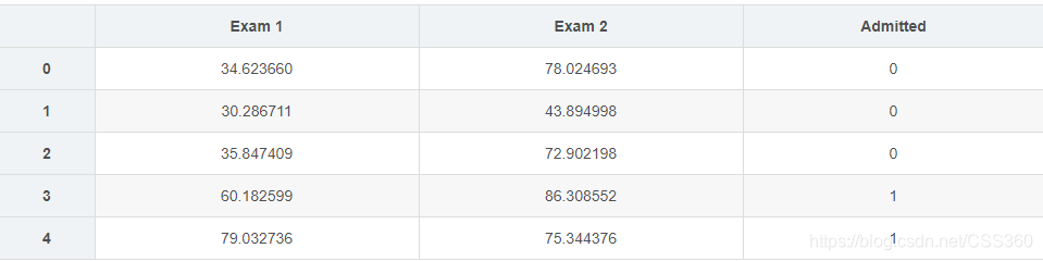
#样本训练数据为申请入学的学生两次测评的成绩，以及最后是否被录取的结果。

data = pd.read_csv('ex2data1.txt', header=None, names=['Exam 1', 'Exam 2', 'Admitted'])
data.head()

positive = data[data['Admitted'].isin([1])]
negative = data[data['Admitted'].isin([0])]

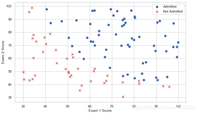
#数据可视化
#创建两个分数的散点图，并使用颜色编码来可视化，如果样本是正的（被接纳）或负的（未被接纳）
fig, ax = plt.subplots(figsize=(10,6))
ax.scatter(positive['Exam 1'], positive['Exam 2'], s=50, c='b', marker='o', label='Admitted')
ax.scatter(negative['Exam 1'], negative['Exam 2'], s=50, c='r', marker='x', label='Not Admitted')
ax.legend()
ax.set_xlabel('Exam 1 Score')
ax.set_ylabel('Exam 2 Score')

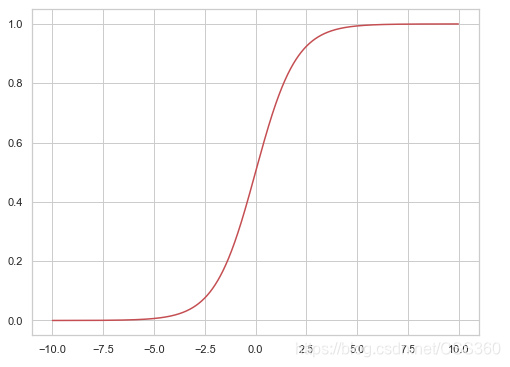
#sigmoid 函数
def sigmoid(z):
    return 1 / (1 + np.exp(-z))


nums = np.arange(-10, 10, step=0.01)

fig, ax = plt.subplots(figsize=(8,6))
ax.plot(nums, sigmoid(nums), 'r')

#代价函数：
def cost(theta, X, y):
    theta = np.matrix(theta)
    X = np.matrix(X)
    y = np.matrix(y)
    first = np.multiply(-y, np.log(sigmoid(X * theta.T)))
    second = np.multiply((1 - y), np.log(1 - sigmoid(X * theta.T)))
    return np.sum(first - second) / (len(X))

#对数据稍作处理，同exercise1
# add a ones column - this makes the matrix multiplication work out easier
data.insert(0, 'Ones', 1)

# set X (training data) and y (target variable)
cols = data.shape[1]
X = data.iloc[:,0:cols-1]
y = data.iloc[:,cols-1:cols]

# convert to numpy arrays and initalize the parameter array theta
X = np.array(X.values)
y = np.array(y.values)
theta = np.zeros(3)

#计算一下初始化参数的cost
cost(theta, X, y)

#gradient descent(梯度下降)
def gradient(theta, X, y):
    theta = np.matrix(theta)
    X = np.matrix(X)
    y = np.matrix(y)
    
    parameters = int(theta.ravel().shape[1])
    grad = np.zeros(parameters)
    
    error = sigmoid(X * theta.T) - y
    
    for i in range(parameters):
        term = np.multiply(error, X[:,i])
        grad[i] = np.sum(term) / len(X)
    
    return grad

#使用 scipy.optimize.minimize 去拟合参数
import scipy.optimize as opt
res = opt.minimize(fun=cost, x0=theta, args=(X, y), method='Newton-CG', jac=gradient)
print(res)

#预测与验证
def predict(theta, X):
    probability = sigmoid(X * theta.T)
    return [1 if x >= 0.5 else 0 for x in probability]

final_theta =np.matrix(res.x)
predictions = predict(final_theta, X)
correct = [1 if ((a == 1 and b == 1) or (a == 0 and b == 0)) else 0 for (a, b) in zip(predictions, y)]
accuracy = (sum(map(int, correct)) % len(correct))
print ('accuracy = {0}%'.format(accuracy))

#寻找决策边界
coef = -(res.x / res.x[2])  # find the equation
print(coef)

positive = data[data['Admitted'].isin([1])]
negative = data[data['Admitted'].isin([0])]

fig, ax = plt.subplots(figsize=(10,6))
ax.scatter(positive['Exam 1'], positive['Exam 2'], s=50, c='b', marker='o', label='Admitted')
ax.scatter(negative['Exam 1'], negative['Exam 2'], s=50, c='r', marker='x', label='Not Admitted')
ax.legend()
ax.set_xlabel('Exam 1 Score')
ax.set_ylabel('Exam 2 Score')

x = np.arange(30,100, step=0.1)
y = coef[0] + coef[1]*x
plt.plot(x, y, 'grey')


'''
第二部分：逻辑回归+正则化
说明：这部分也要用到上一部分中的函数，所以要一起运行
'''


#正则化逻辑回归
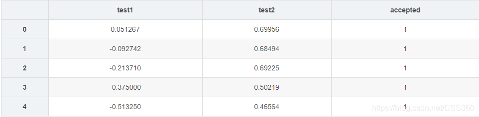
data2 = pd.read_csv('ex2data2.txt',header=None,names = ['test1','test2','accepted'])
data2.head()

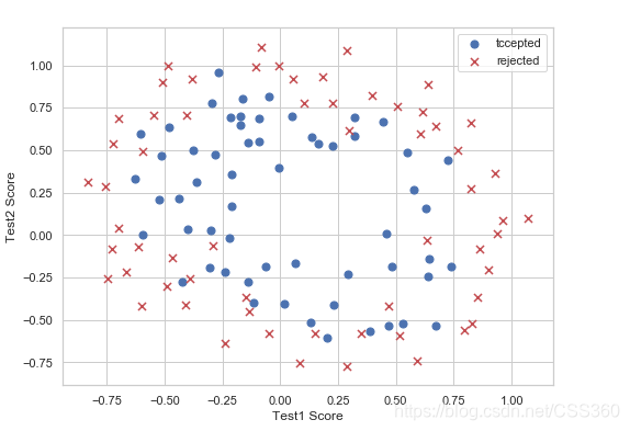
positive = data2[data2['accepted'].isin([1])]
negative = data2[data2['accepted'].isin([0])]

fig, ax = plt.subplots(figsize=(8,6))
ax.scatter(positive['test1'], positive['test2'], s=50, c='b', marker='o', label='tccepted')
ax.scatter(negative['test1'], negative['test2'], s=50, c='r', marker='x', label='rejected')
ax.legend()
ax.set_xlabel('Test1 Score')
ax.set_ylabel('Test2 Score')

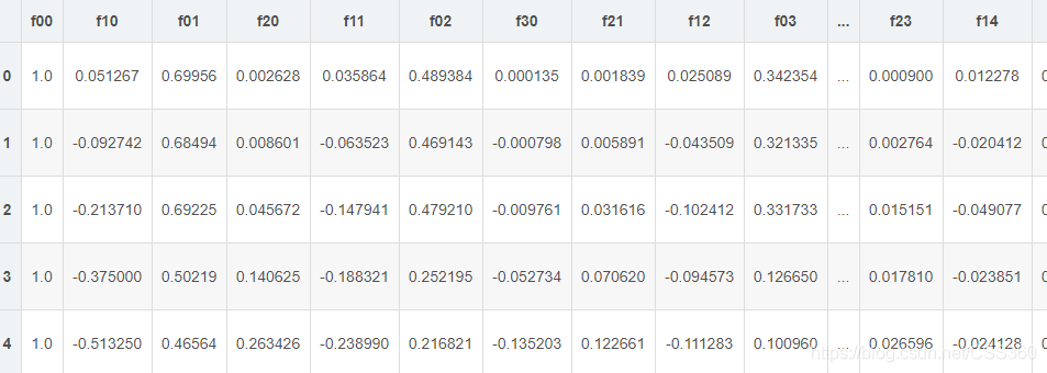
#feature mapping（特征映射）
def feature_mapping(x, y, power, as_ndarray=False):

    data = {"f{}{}".format(i - p, p): np.power(x, i - p) * np.power(y, p)
                for i in np.arange(power + 1)
                for p in np.arange(i + 1)
            }

    if as_ndarray:
        return pd.DataFrame(data).as_matrix()
    else:
        return pd.DataFrame(data)
    
x1 = np.array(data2.test1)
x2 = np.array(data2.test2)

d = feature_mapping(x1, x2, power=6)
print(d.shape)
d.head()

# set X and y (remember from above that we moved the label to column 0)
cols = d.shape[1]
X2 = d.iloc[:,0:cols]
y2 = data2.iloc[:,-1]

# convert to numpy arrays and initalize the parameter array theta
X2 = np.array(X2.values)
y2 = np.array(y2.values)
theta2 = np.zeros(d.shape[1])
print(X2.shape)

#regularized cost（正则化代价函数）
def regularized_cost(theta, X, y, l = 1):
#     '''you don't penalize theta_0'''
    theta_j1_to_n = theta[1:]
    regularized_term = (l / (2 * len(X))) * np.power(theta_j1_to_n, 2).sum()

    return cost(theta, X, y) + regularized_term
#正则化代价函数
regularized_cost(theta2, X2, y2)

#regularized gradient(正则化梯度)
def gradientReg(theta, X, y, l = 1):
    theta = np.matrix(theta)
    X = np.matrix(X)
    y = np.matrix(y)
    
    parameters = int(theta.ravel().shape[1])
    grad = np.zeros(parameters)
    
    error = sigmoid(X * theta.T) - y
    
    for i in range(parameters):
        term = np.multiply(error, X[:,i])
        
        if (i == 0):
            grad[i] = np.sum(term) / len(X)
        else:
            grad[i] = (np.sum(term) / len(X)) + ((l/ len(X)) * theta[:,i])
    
    return grad

gradientReg(theta2,X2,y2,l=1)

#使用 scipy.optimize.minimize 去拟合参数

import scipy.optimize as opt
#print('init cost = {}'.format(regularized_cost(theta, X2, y2)))

res = opt.minimize(fun=regularized_cost, x0=theta2, args=(X2, y2), method='Newton-CG', jac=gradientReg)
print(res)

theta_min =np.matrix(res.x)
predictions = predict(theta_min, X2)
correct = [1 if ((a == 1 and b == 1) or (a == 0 and b == 0)) else 0 for (a, b) in zip(predictions, y2)]
accuracy = (sum(map(int, correct)) % len(correct))
print ('accuracy = {0}%'.format(accuracy))

#调用sklearn的线性回归包

from sklearn import linear_model
model = linear_model.LogisticRegression(penalty='l2', C=1.0)
model.fit(X2, y2.ravel())

linear_model.LogisticRegression(C=1.0, class_weight=None, dual=False, fit_intercept=True,
          intercept_scaling=1, max_iter=100, multi_class='warn',
          n_jobs=None, penalty='l2', random_state=None, solver='warn',
          tol=0.0001, verbose=0, warm_start=False)

print(model.score(X2, y2))

（2）实验结果

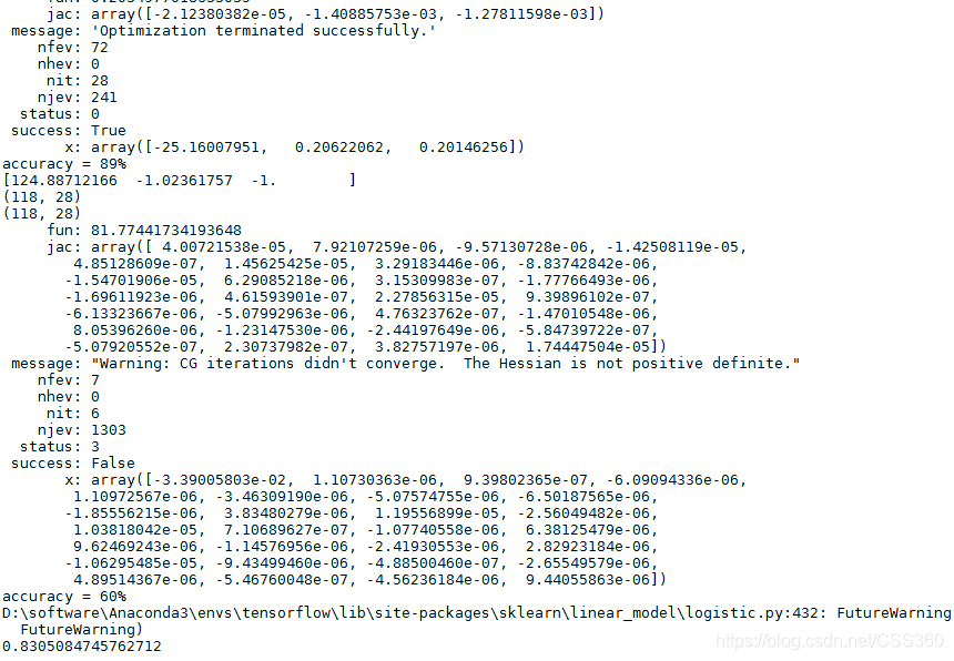
（3）关键部分详细讲解

数据分布

data = pd.read_csv('ex2data1.txt', header=None, names=['Exam 1', 'Exam 2', 'Admitted'])
data.head()

数据可视化

Sigmoid函数

一般我们比较常见的Sigmoid函数为： $g(z) = \frac{1}{1 + e^{-z}}$ ，在这里我们假设函数为 $h_{\theta } (x)= \frac{1}{1 + e^{-\theta ^{T}X}}$

def sigmoid(z):
    return 1 / (1 + np.exp(-z))

损失函数（关于此函数怎么来的请看链接）

$J(\theta ) = \frac{1}{m}\sum_{i = 1}^{m} \left [ -y^{(i)}log(h_{\theta }(x^{(i)})) - (1 - y^{(i)})log(1 - h_{\theta }(x^{(i)})) \right ]$

def cost(theta, X, y):
    theta = np.matrix(theta)
    X = np.matrix(X)
    y = np.matrix(y)
    first = np.multiply(-y, np.log(sigmoid(X * theta.T)))
    second = np.multiply((1 - y), np.log(1 - sigmoid(X * theta.T)))
    return np.sum(first - second) / (len(X))

gradient descent(梯度下降)

在这里使用批量梯度下降方法，并将其转化为向量方法，则 $\frac{1}{m}X^{T}(Sigmoid(X^{T}\theta ) - y)$ 转化为 $\frac{\partial J(\theta)}{\partial \theta _{j}} = \frac{1}{m}\sum_{i =1}^{m}(h_{\theta}(x^{(i)}) - y^{i})x_{j}^{i}$

#计算一个梯度步长
def gradient(theta, X, y):
    theta = np.matrix(theta)
    X = np.matrix(X)
    y = np.matrix(y)
    
    parameters = int(theta.ravel().shape[1])
    grad = np.zeros(parameters)
    
    error = sigmoid(X * theta.T) - y
    
    for i in range(parameters):
        term = np.multiply(error, X[:,i])
        grad[i] = np.sum(term) / len(X)
    
    return grad

第二部分：正则化逻辑回归

数据格式

数据可视化

feature mapping（特征映射）

$mapFeature = \begin{bmatrix} 1\\ x_{1}\\ x_{2}\\ x_{1}^{2}\\ x_{1}x_{2}\\ x_{2}^{2}\\ x_{1}^{3}\\ x_{1}*x_{2}^{5} \\ x_{1}*x_{2}^{6} \\ \end{bmatrix}$

def feature_mapping(x, y, power, as_ndarray=False):

    data = {"f{}{}".format(i - p, p): np.power(x, i - p) * np.power(y, p)
                for i in np.arange(power + 1)
                for p in np.arange(i + 1)
            }

    if as_ndarray:
        return pd.DataFrame(data).as_matrix()
    else:
        return pd.DataFrame(data)

特征映射对应的数据：

regularized cost（正则化代价函数）

$J(\theta ) = \frac{1}{m}\sum_{i = 1}^{m} \left [ -y^{(i)}log(h_{\theta }(x^{(i)})) - (1 - y^{(i)})log(1 - h_{\theta }(x^{(i)})) \right ] + \frac{\lambda }{2m}\sum_{j =1}^{n}\theta _{j}^{2}$

def regularized_cost(theta, X, y, l = 1):
#     '''you don't penalize theta_0'''
    theta_j1_to_n = theta[1:]
    regularized_term = (l / (2 * len(X))) * np.power(theta_j1_to_n, 2).sum()

    return cost(theta, X, y) + regularized_term
#正则化代价函数

regularized gradient(正则化梯度)

$\frac{\partial J(\theta)}{\partial \theta _{j}} = \frac{1}{m}\sum_{i =1}^{m}(h_{\theta}(x^{(i)}) - y^{i})x_{j}^{i} + \frac{\lambda }{m}\theta _{j} \begin{matrix}\end{matrix} \begin{matrix} \end{matrix}$ $j\geq 1$

def gradientReg(theta, X, y, l = 1):
    theta = np.matrix(theta)
    X = np.matrix(X)
    y = np.matrix(y)
    
    parameters = int(theta.ravel().shape[1])
    grad = np.zeros(parameters)
    
    error = sigmoid(X * theta.T) - y
    
    for i in range(parameters):
        term = np.multiply(error, X[:,i])
        
        if (i == 0):
            grad[i] = np.sum(term) / len(X)
        else:
            grad[i] = (np.sum(term) / len(X)) + ((l/ len(X)) * theta[:,i])
    
    return grad

独孤九剑-风清扬

发布了149 篇原创文章 · 获赞 22 · 访问量 4万+

私信关注

正则化从理论到实践专题

猜你喜欢