CNN入门：通俗理解卷积神经网络

 通俗理解卷积神经网络（cs231n与5月dl班课程笔记）

1 前言

    2012年我在北京组织过8期machine learning读书会，那时“机器学习”非常火，很多人都对其抱有巨大的热情。当我2013年再次来到北京时，有一个词似乎比“机器学习”更火，那就是“深度学习”。

    本博客内写过一些机器学习相关的文章，但上一篇技术文章“LDA主题模型”还是写于2014年11月份，毕竟自2015年开始创业做在线教育后，太多的杂事、琐碎事，让我一直想再写点技术性文章但每每恨时间抽不开。然由于公司在不断开机器学习、深度学习等相关的在线课程，耳濡目染中，总会顺带着学习学习。

    我虽不参与讲任何课程（我所在公司“七月在线”的所有在线课程都是由目前讲师团队的60位讲师讲），但依然可以用最最小白的方式 把一些初看复杂的东西抽丝剥茧的通俗写出来。这算重写技术博客的价值所在。

    在dl中，有一个很重要的概念，就是卷积神经网络CNN，基本是入门dl必须搞懂的东西。本文基本根据斯坦福的机器学习公开课、cs231n、与七月在线寒小阳讲的5月dl班第4次课CNN与常用框架视频所写，是一篇课程笔记。

    一开始本文只是想重点讲下CNN中的卷积操作具体是怎么计算怎么操作的，但后面不断补充，包括增加不少自己的理解，故写成了关于卷积神经网络的通俗导论性的文章。有何问题，欢迎不吝指正。

2 人工神经网络

2.1 神经元

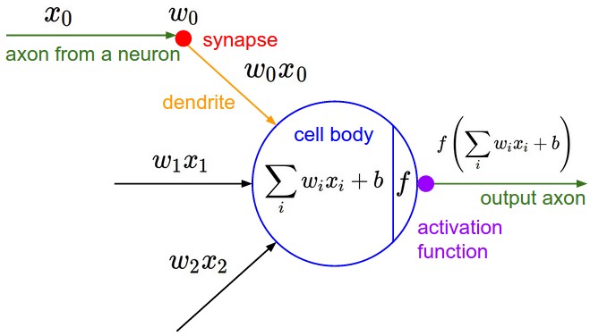
    神经网络由大量的神经元相互连接而成。每个神经元接受线性组合的输入后，最开始只是简单的线性加权，后来给每个神经元加上了非线性的激活函数，从而进行非线性变换后输出。每两个神经元之间的连接代表加权值，称之为权重（weight）。不同的权重和激活函数，则会导致神经网络不同的输出。

    举个手写识别的例子，给定一个未知数字，让神经网络识别是什么数字。此时的神经网络的输入由一组被输入图像的像素所激活的输入神经元所定义。在通过非线性激活函数进行非线性变换后，神经元被激活然后被传递到其他神经元。重复这一过程，直到最后一个输出神经元被激活。从而识别当前数字是什么字。

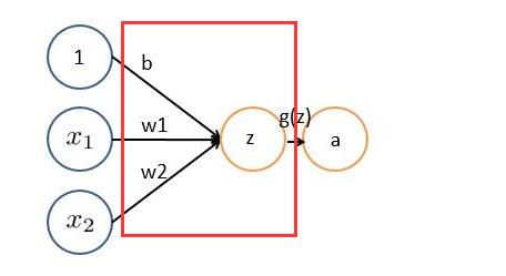
    神经网络的每个神经元如下

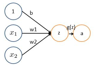
    基本wx + b的形式，其中

• 、表示输入向量
• 、为权重，几个输入则意味着有几个权重，即每个输入都被赋予一个权重
• b为偏置bias
• g(z) 为激活函数
• a 为输出

    如果只是上面这样一说，估计以前没接触过的十有八九又必定迷糊了。事实上，上述简单模型可以追溯到20世纪50/60年代的感知器，可以把感知器理解为一个根据不同因素、以及各个因素的重要性程度而做决策的模型。

    举个例子，这周末北京有一草莓音乐节，那去不去呢？决定你是否去有二个因素，这二个因素可以对应二个输入，分别用x1、x2表示。此外，这二个因素对做决策的影响程度不一样，各自的影响程度用权重w1、w2表示。一般来说，音乐节的演唱嘉宾会非常影响你去不去，唱得好的前提下 即便没人陪同都可忍受，但如果唱得不好还不如你上台唱呢。所以，我们可以如下表示：

• ：是否有喜欢的演唱嘉宾。 = 1 你喜欢这些嘉宾， = 0 你不喜欢这些嘉宾。嘉宾因素的权重 = 7
• ：是否有人陪你同去。 = 1 有人陪你同去， = 0 没人陪你同去。是否有人陪同的权重 = 3。

    这样，咱们的决策模型便建立起来了：g(z) = g( * + * + b )，g表示激活函数，这里的b可以理解成 为更好达到目标而做调整的偏置项。

    一开始为了简单，人们把激活函数定义成一个线性函数，即对于结果做一个线性变化，比如一个简单的线性激活函数是g(z) = z，输出都是输入的线性变换。后来实际应用中发现，线性激活函数太过局限，于是人们引入了非线性激活函数。

2.2 激活函数

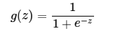
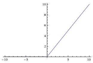
    常用的非线性激活函数有sigmoid、tanh、relu等等，前两者sigmoid/tanh比较常见于全连接层，后者relu常见于卷积层。这里先简要介绍下最基础的sigmoid函数（btw，在本博客中SVM那篇文章开头有提过）。

    sigmoid的函数表达式如下

    其中z是一个线性组合，比如z可以等于：b + * + *。通过代入很大的正数或很小的负数到g(z)函数中可知，其结果趋近于0或1。

    因此，sigmoid函数g(z)的图形表示如下（ 横轴表示定义域z，纵轴表示值域g(z) ）：

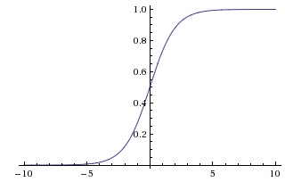
    也就是说，sigmoid函数的功能是相当于把一个实数压缩至0到1之间。当z是非常大的正数时，g(z)会趋近于1，而z是非常小的负数时，则g(z)会趋近于0。

    压缩至0到1有何用处呢？用处是这样一来便可以把激活函数看作一种“分类的概率”，比如激活函数的输出为0.9的话便可以解释为90%的概率为正样本。

    举个例子，如下图（图引自Stanford机器学习公开课）

    z = b + * + *，其中b为偏置项 假定取-30，、都取为20

• 如果 = 0  = 0，则z = -30，g(z) = 1/( 1 + e^-z )趋近于0。此外，从上图sigmoid函数的图形上也可以看出，当z=-30的时候，g(z)的值趋近于0
• 如果 = 0 = 1，或 =1 = 0，则z = b + * + * = -30 + 20 = -10，同样，g(z)的值趋近于0
• 如果 = 1 = 1，则z = b + * + * = -30 + 20*1 + 20*1 = 10，此时，g(z)趋近于1。

    换言之，只有和都取1的时候，g(z)→1，判定为正样本；或取0的时候，g(z)→0，判定为负样本，如此达到分类的目的。

2.3 神经网络

    将下图的这种单个神经元

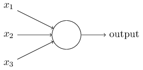
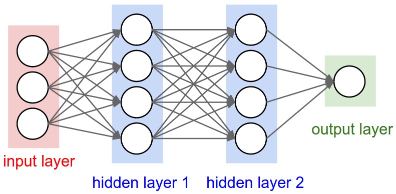
    组织在一起，便形成了神经网络。下图便是一个三层神经网络结构

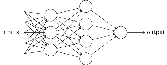
    上图中最左边的原始输入信息称之为输入层，最右边的神经元称之为输出层（上图中输出层只有一个神经元），中间的叫隐藏层。

    啥叫输入层、输出层、隐藏层呢？

• 输入层（Input layer），众多神经元（Neuron）接受大量非线形输入讯息。输入的讯息称为输入向量。
• 输出层（Output layer），讯息在神经元链接中传输、分析、权衡，形成输出结果。输出的讯息称为输出向量。
• 隐藏层（Hidden layer），简称“隐层”，是输入层和输出层之间众多神经元和链接组成的各个层面。如果有多个隐藏层，则意味着多个激活函数。

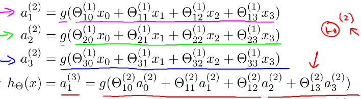
    同时，每一层都可能由单个或多个神经元组成，每一层的输出将会作为下一层的输入数据。比如下图中间隐藏层来说，隐藏层的3个神经元a1、a2、a3皆各自接受来自多个不同权重的输入（因为有x1、x2、x3这三个输入，所以a1 a2 a3都会接受x1 x2 x3各自分别赋予的权重，即几个输入则几个权重），接着，a1、a2、a3又在自身各自不同权重的影响下 成为的输出层的输入，最终由输出层输出最终结果。

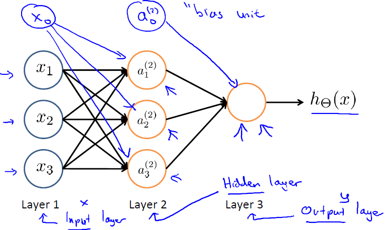
    上图（图引自Stanford机器学习公开课）中

• 表示第j层第i个单元的激活函数/神经元
• 表示从第j层映射到第j+1层的控制函数的权重矩阵 

    此外， 输入层和隐藏层都存在一个偏置（bias unit)，所以上图中也增加了偏置项：x0、a0。针对上图，有如下公式

    此外，上文中讲的都是一层隐藏层，但实际中也有多层隐藏层的，即输入层和输出层中间夹着数层隐藏层，层和层之间是全连接的结构，同一层的神经元之间没有连接。

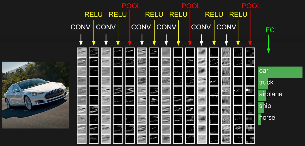
3 卷积神经网络之层级结构

   cs231n课程里给出了卷积神经网络各个层级结构，如下图

    上图中CNN要做的事情是：给定一张图片，是车还是马未知，是什么车也未知，现在需要模型判断这张图片里具体是一个什么东西，总之输出一个结果：如果是车 那是什么车

    所以

• 最左边是数据输入层，对数据做一些处理，比如去均值（把输入数据各个维度都中心化为0，避免数据过多偏差，影响训练效果）、归一化（把所有的数据都归一到同样的范围）、PCA/白化等等。CNN只对训练集做“去均值”这一步。

    中间是

• CONV：卷积计算层，线性乘积 求和。
• RELU：激励层，上文2.2节中有提到：ReLU是激活函数的一种。
• POOL：池化层，简言之，即取区域平均或最大。

    最右边是

• FC：全连接层

    这几个部分中，卷积计算层是CNN的核心，下文将重点阐述。

4 CNN之卷积计算层

4.1 CNN怎么进行识别

    当我们给定一个"X"的图案，计算机怎么识别这个图案就是“X”呢？一个可能的办法就是计算机存储一张标准的“X”图案，然后把需要识别的未知图案跟标准"X"图案进行比对，如果二者一致，则判定未知图案即是一个"X"图案。

    而且即便未知图案可能有一些平移或稍稍变形，依然能辨别出它是一个X图案。如此，CNN是把未知图案和标准X图案一个局部一个局部的对比，如下图所示 [图来自参考文案25]

    而未知图案的局部和标准X图案的局部一个一个比对时的计算过程，便是卷积操作。卷积计算结果为1表示匹配，否则不匹配。

    接下来，我们来了解下什么是卷积操作。

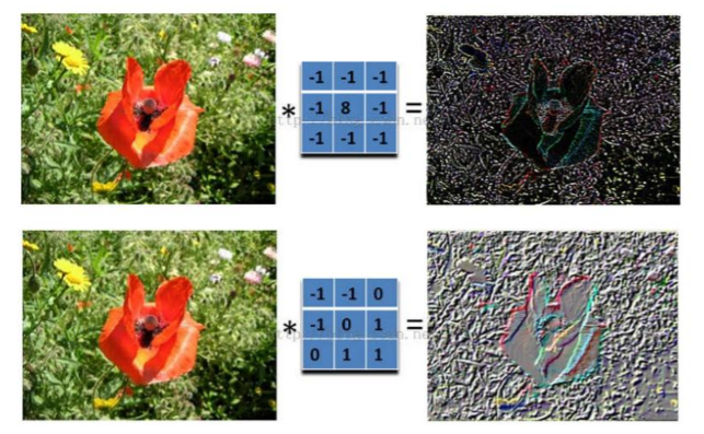
4.2 什么是卷积

    对图像（不同的数据窗口数据）和滤波矩阵（一组固定的权重：因为每个神经元的多个权重固定，所以又可以看做一个恒定的滤波器filter）做 内积（逐个元素相乘再求和）的操作就是所谓的『卷积』操作，也是卷积神经网络的名字来源。

    非严格意义上来讲，下图中红框框起来的部分便可以理解为一个滤波器，即带着一组固定权重的神经元。多个滤波器叠加便成了卷积层。

    OK，举个具体的例子。比如下图中，图中左边部分是原始输入数据，图中中间部分是滤波器filter，图中右边是输出的新的二维数据。

    分解下上图

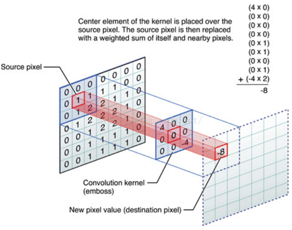
对应位置上是数字先相乘后相加 =

    中间滤波器filter与数据窗口做内积，其具体计算过程则是：4*0 + 0*0 + 0*0 + 0*0 + 0*1 + 0*1 + 0*0 + 0*1 + -4*2 = -8

4.3 图像上的卷积

    在下图对应的计算过程中，输入是一定区域大小(width*height)的数据，和滤波器filter（带着一组固定权重的神经元）做内积后等到新的二维数据。

    具体来说，左边是图像输入，中间部分就是滤波器filter（带着一组固定权重的神经元），不同的滤波器filter会得到不同的输出数据，比如颜色深浅、轮廓。相当于如果想提取图像的不同特征，则用不同的滤波器filter，提取想要的关于图像的特定信息：颜色深浅或轮廓。

    如下图所示

  

4.4 GIF动态卷积图

    在CNN中， 滤波器filter（带着一组固定权重的神经元）对局部输入数据进行卷积计算。每计算完一个数据窗口内的局部数据后，数据窗口不断平移滑动，直到计算完所有数据。这个过程中，有这么几个参数： 
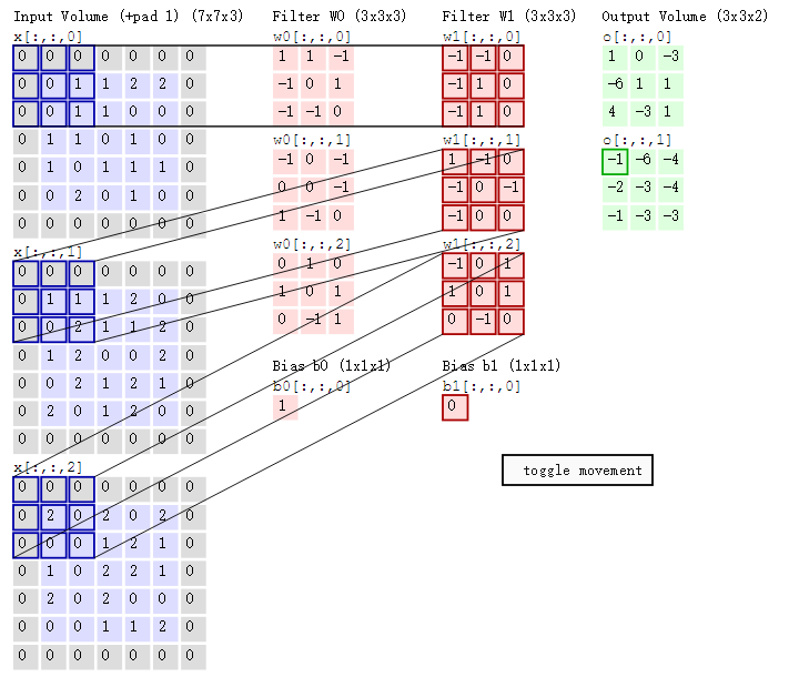
　　a.  深度depth ：神经元个数，决定输出的depth厚度。同时代表滤波器个数。
　　b.  步长stride ：决定滑动多少步可以到边缘。

　　c.  填充值zero-padding ：在外围边缘补充若干圈0，方便从初始位置以步长为单位可以刚好滑倒末尾位置，通俗地讲就是为了总长能被步长整除。 

　　  

    cs231n课程中有一张卷积动图，貌似是用d3js 和一个util 画的，我 根据cs231n的卷积动图依次截取了18张图，然后用一gif 制图工具制作了一gif 动态卷积图。如下gif 图所示

    可以看到：

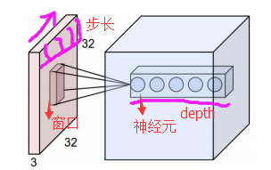
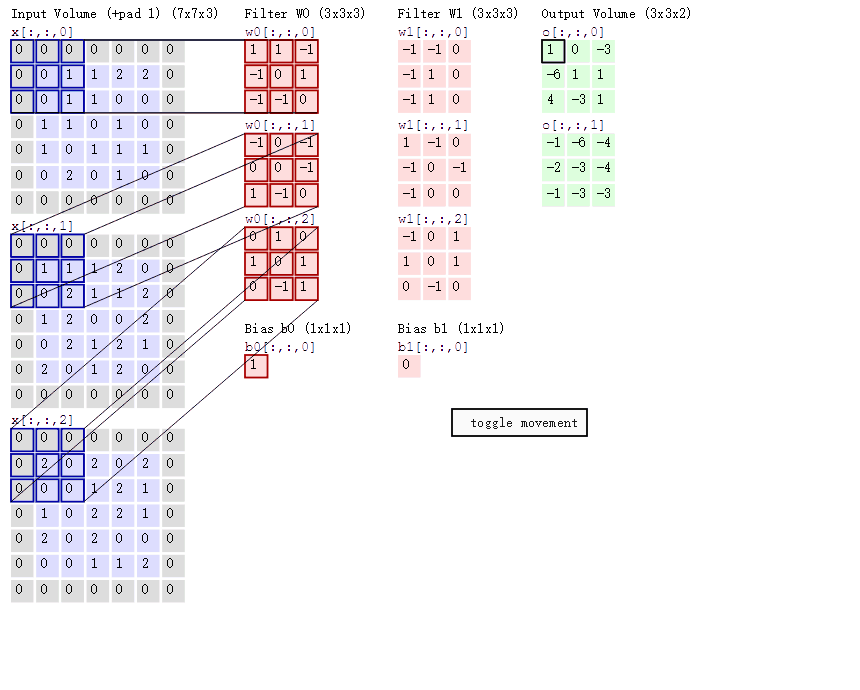
• 两个神经元，即depth=2，意味着有两个滤波器。
• 数据窗口每次移动两个步长取3*3的局部数据，即stride=2。
• zero-padding=1。

    然后分别以两个滤波器filter为轴滑动数组进行卷积计算，得到两组不同的结果。

    如果初看上图，可能不一定能立马理解啥意思，但结合上文的内容后，理解这个动图已经不是很困难的事情：

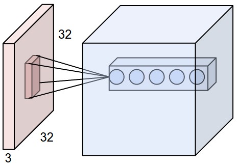
• 左边是输入（7*7*3中，7*7代表图像的像素/长宽，3代表R、G、B 三个颜色通道）
• 中间部分是两个不同的滤波器Filter w0、Filter w1
• 最右边则是两个不同的输出

    随着左边数据窗口的平移滑动，滤波器Filter w0 / Filter w1对不同的局部数据进行卷积计算。

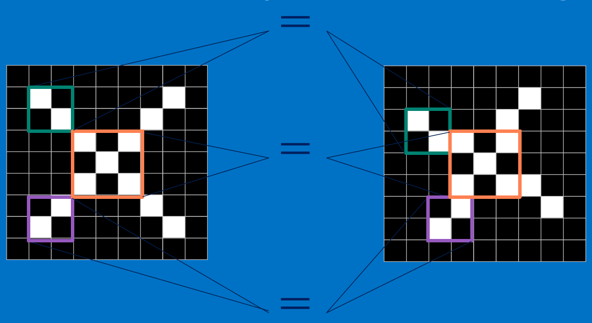
    值得一提的是：

1. 左边数据在变化，每次滤波器都是针对某一局部的数据窗口进行卷积，这就是所谓的CNN中的局部感知机制。

• 打个比方，滤波器就像一双眼睛，人类视角有限，一眼望去，只能看到这世界的局部。如果一眼就看到全世界，你会累死，而且一下子接受全世界所有信息，你大脑接收不过来。当然，即便是看局部，针对局部里的信息人类双眼也是有偏重、偏好的。比如看美女，对脸、胸、腿是重点关注，所以这3个输入的权重相对较大。

与此同时，数据窗口滑动，导致输入在变化，但中间滤波器Filter w0的权重（即每个神经元连接数据窗口的权重）是固定不变的，这个权重不变即所谓的CNN中的 参数（权重）共享机制。

• 再打个比方，某人环游全世界，所看到的信息在变，但采集信息的双眼不变。btw，不同人的双眼 看同一个局部信息 所感受到的不同，即一千个读者有一千个哈姆雷特，所以不同的滤波器 就像不同的双眼，不同的人有着不同的反馈结果。

    我第一次看到上面这个动态图的时候，只觉得很炫，另外就是据说计算过程是“相乘后相加”，但到底具体是个怎么相乘后相加的计算过程 则无法一眼看出，网上也没有一目了然的计算过程。本文来细究下。

    首先，我们来分解下上述动图，如下图

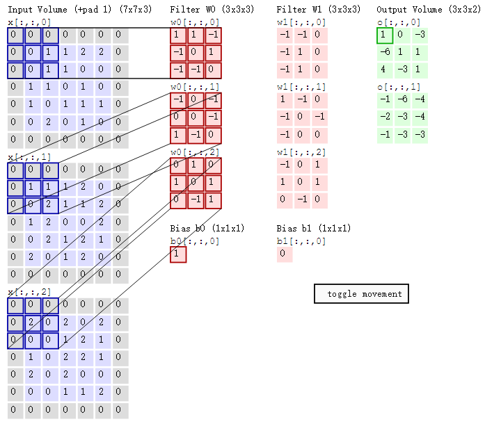
    接着，我们细究下上图的具体计算过程。即上图中的输出结果1具体是怎么计算得到的呢？其实，类似wx + b，w对应滤波器Filter w0，x对应不同的数据窗口，b对应Bias b0，相当于滤波器Filter w0与一个个数据窗口相乘再求和后，最后加上Bias b0得到输出结果1，如下过程所示：

1* 0 + 1*0 + -1*0 

+

-1*0 + 0*0 + 1*1

+

-1*0 + -1*0 + 0*1

+

-1*0 + 0*0 + -1*0

+

0*0 + 0*1 + -1*1

+

1*0 + -1*0 + 0*2

+

0*0 + 1*0 + 0*0

+

1*0 + 0*2 + 1*0

+

0*0 + -1*0 + 1*0

+

 

1

=

1

    然后滤波器Filter w0固定不变，数据窗口向右移动2步，继续做内积计算，得到0的输出结果

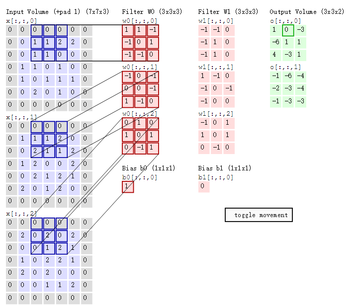
    最后，换做另外一个不同的滤波器Filter w1、不同的偏置Bias b1，再跟图中最左边的数据窗口做卷积，可得到另外一个不同的输出。

5 CNN之激励层与池化层

5.1 ReLU激励层

    2.2节介绍了激活函数sigmoid，但实际梯度下降中，sigmoid容易饱和、造成终止梯度传递，且没有0中心化。咋办呢，可以尝试另外一个激活函数：ReLU，其图形表示如下

    ReLU的优点是收敛快，求梯度简单。

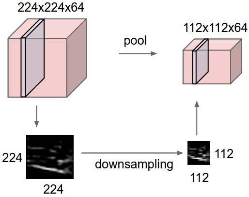
5.2 池化pool层

    前头说了，池化，简言之，即取区域平均或最大，如下图所示（图引自cs231n）

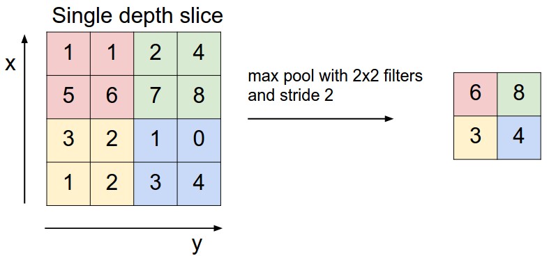
    上图所展示的是取区域最大，即上图左边部分中 左上角2x2的矩阵中6最大，右上角2x2的矩阵中8最大，左下角2x2的矩阵中3最大，右下角2x2的矩阵中4最大，所以得到上图右边部分的结果：6 8 3 4。很简单不是？

6 参考文献及推荐阅读

1. 人工神经网络wikipedia
2. 斯坦福机器学习公开课
3. http://neuralnetworksanddeeplearning.com/
   
4. 雨石 卷积神经网络：http://blog.csdn.net/stdcoutzyx/article/details/41596663
   
5. cs231n 神经网络结构与神经元激励函数：http://cs231n.github.io/neural-networks-1/，中译版
   
6. cs231n 卷积神经网络：http://cs231n.github.io/convolutional-networks/
7. 七月在线寒老师讲的5月dl班第4次课CNN与常用框架视频，已经剪切部分放在七月在线官网：julyedu.com
8. 七月在线5月深度学习班第5课CNN训练注意事项部分视频：https://www.julyedu.com/video/play/42/207
9. 七月在线5月深度学习班：https://www.julyedu.com/course/getDetail/37
10. 七月在线5月深度学习班课程笔记——No.4《CNN与常用框架》：http://blog.csdn.net/joycewyj/article/details/51792477
11. 七月在线6月数据数据挖掘班第7课视频：数据分类与排序
12. 手把手入门神经网络系列(1)_从初等数学的角度初探神经网络：http://blog.csdn.net/han_xiaoyang/article/details/50100367
    
13. 深度学习与计算机视觉系列(6)_神经网络结构与神经元激励函数：http://blog.csdn.net/han_xiaoyang/article/details/50447834
    
14. 深度学习与计算机视觉系列(10)_细说卷积神经网络：http://blog.csdn.net/han_xiaoyang/article/details/50542880
    
15. zxy 图像卷积与滤波的一些知识点：http://blog.csdn.net/zouxy09/article/details/49080029
16. zxy 深度学习CNN笔记：http://blog.csdn.net/zouxy09/article/details/8781543/
17. http://www.wildml.com/2015/11/understanding-convolutional-neural-networks-for-nlp/，中译版
    
18. 《神经网络与深度学习》中文讲义：http://vdisk.weibo.com/s/A_pmE4iIPs9D
19. ReLU与sigmoid/tanh的区别：https://www.zhihu.com/question/29021768
20. CNN、RNN、DNN内部网络结构区别：https://www.zhihu.com/question/34681168
21. 理解卷积：https://www.zhihu.com/question/22298352
22. 神经网络与深度学习简史：1 感知机和BP算法、4 深度学习的伟大复兴
23. 在线制作gif 动图：http://www.tuyitu.com/photoshop/gif.htm
24. 支持向量机通俗导论（理解SVM的三层境界）
    
25. CNN究竟是怎样一步一步工作的？ 本博客把卷积操作具体怎么个计算过程写清楚了，但这篇把为何要卷积操作也写清楚了，而且配偶图非常形象，甚赞。

参考：https://blog.csdn.net/v_july_v/article/details/51812459

参考原文链接：CS231n Convolutional Neural Networks for Visual Recognition

Table of Contents:

• Architecture Overview
• ConvNet Layers
  • Convolutional Layer
  • Pooling Layer
  • Normalization Layer
  • Fully-Connected Layer
  • Converting Fully-Connected Layers to Convolutional Layers
• ConvNet Architectures
  • Layer Patterns
  • Layer Sizing Patterns
  • Case Studies (LeNet / AlexNet / ZFNet / GoogLeNet / VGGNet)
  • Computational Considerations
• Additional References

Convolutional Neural Networks (CNNs / ConvNets)

Convolutional Neural Networks are very similar to ordinary Neural Networks from the previous chapter: they are made up of neurons that have learnable weights and biases. Each neuron receives some inputs, performs a dot product and optionally follows it with a non-linearity. The whole network still expresses a single differentiable score function: from the raw image pixels on one end to class scores at the other. And they still have a loss function (e.g. SVM/Softmax) on the last (fully-connected) layer and all the tips/tricks we developed for learning regular Neural Networks still apply.

So what does change? ConvNet architectures make the explicit assumption that the inputs are images, which allows us to encode certain properties into the architecture. These then make the forward function more efficient to implement and vastly reduce the amount of parameters in the network.

Architecture Overview

Recall: Regular Neural Nets. As we saw in the previous chapter, Neural Networks receive an input (a single vector), and transform it through a series of hidden layers. Each hidden layer is made up of a set of neurons, where each neuron is fully connected to all neurons in the previous layer, and where neurons in a single layer function completely independently and do not share any connections. The last fully-connected layer is called the “output layer” and in classification settings it represents the class scores.

Regular Neural Nets don’t scale well to full images. In CIFAR-10, images are only of size 32x32x3 (32 wide, 32 high, 3 color channels), so a single fully-connected neuron in a first hidden layer of a regular Neural Network would have 32*32*3 = 3072 weights. This amount still seems manageable, but clearly this fully-connected structure does not scale to larger images. For example, an image of more respectable size, e.g. 200x200x3, would lead to neurons that have 200*200*3 = 120,000 weights. Moreover, we would almost certainly want to have several such neurons, so the parameters would add up quickly! Clearly, this full connectivity is wasteful and the huge number of parameters would quickly lead to overfitting.

3D volumes of neurons. Convolutional Neural Networks take advantage of the fact that the input consists of images and they constrain the architecture in a more sensible way. In particular, unlike a regular Neural Network, the layers of a ConvNet have neurons arranged in 3 dimensions: width, height, depth. (Note that the word depth here refers to the third dimension of an activation volume, not to the depth of a full Neural Network, which can refer to the total number of layers in a network.) For example, the input images in CIFAR-10 are an input volume of activations, and the volume has dimensions 32x32x3 (width, height, depth respectively). As we will soon see, the neurons in a layer will only be connected to a small region of the layer before it, instead of all of the neurons in a fully-connected manner. Moreover, the final output layer would for CIFAR-10 have dimensions 1x1x10, because by the end of the ConvNet architecture we will reduce the full image into a single vector of class scores, arranged along the depth dimension. Here is a visualization:

Left: A regular 3-layer Neural Network. Right: A ConvNet arranges its neurons in three dimensions (width, height, depth), as visualized in one of the layers. Every layer of a ConvNet transforms the 3D input volume to a 3D output volume of neuron activations. In this example, the red input layer holds the image, so its width and height would be the dimensions of the image, and the depth would be 3 (Red, Green, Blue channels).

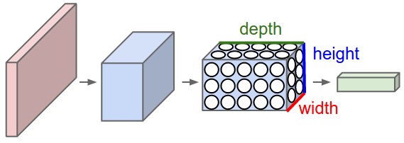
A ConvNet is made up of Layers. Every Layer has a simple API: It transforms an input 3D volume to an output 3D volume with some differentiable function that may or may not have parameters.

Layers used to build ConvNets

As we described above, a simple ConvNet is a sequence of layers, and every layer of a ConvNet transforms one volume of activations to another through a differentiable function. We use three main types of layers to build ConvNet architectures: Convolutional Layer, Pooling Layer, and Fully-Connected Layer (exactly as seen in regular Neural Networks). We will stack these layers to form a full ConvNet architecture.

Example Architecture: Overview. We will go into more details below, but a simple ConvNet for CIFAR-10 classification could have the architecture [INPUT - CONV - RELU - POOL - FC]. In more detail:

• INPUT [32x32x3] will hold the raw pixel values of the image, in this case an image of width 32, height 32, and with three color channels R,G,B.
• CONV layer will compute the output of neurons that are connected to local regions in the input, each computing a dot product between their weights and a small region they are connected to in the input volume. This may result in volume such as [32x32x12] if we decided to use 12 filters.
• RELU layer will apply an elementwise activation function, such as the max(0,x)

• thresholding at zero. This leaves the size of the volume unchanged ([32x32x12]).
• POOL layer will perform a downsampling operation along the spatial dimensions (width, height), resulting in volume such as [16x16x12].
• FC (i.e. fully-connected) layer will compute the class scores, resulting in volume of size [1x1x10], where each of the 10 numbers correspond to a class score, such as among the 10 categories of CIFAR-10. As with ordinary Neural Networks and as the name implies, each neuron in this layer will be connected to all the numbers in the previous volume.

In this way, ConvNets transform the original image layer by layer from the original pixel values to the final class scores. Note that some layers contain parameters and other don’t. In particular, the CONV/FC layers perform transformations that are a function of not only the activations in the input volume, but also of the parameters (the weights and biases of the neurons). On the other hand, the RELU/POOL layers will implement a fixed function. The parameters in the CONV/FC layers will be trained with gradient descent so that the class scores that the ConvNet computes are consistent with the labels in the training set for each image.

In summary:

• A ConvNet architecture is in the simplest case a list of Layers that transform the image volume into an output volume (e.g. holding the class scores)
• There are a few distinct types of Layers (e.g. CONV/FC/RELU/POOL are by far the most popular)
• Each Layer accepts an input 3D volume and transforms it to an output 3D volume through a differentiable function
• Each Layer may or may not have parameters (e.g. CONV/FC do, RELU/POOL don’t)
• Each Layer may or may not have additional hyperparameters (e.g. CONV/FC/POOL do, RELU doesn’t)

The activations of an example ConvNet architecture. The initial volume stores the raw image pixels (left) and the last volume stores the class scores (right). Each volume of activations along the processing path is shown as a column. Since it's difficult to visualize 3D volumes, we lay out each volume's slices in rows. The last layer volume holds the scores for each class, but here we only visualize the sorted top 5 scores, and print the labels of each one. The full web-based demo is shown in the header of our website. The architecture shown here is a tiny VGG Net, which we will discuss later.

We now describe the individual layers and the details of their hyperparameters and their connectivities.

Convolutional Layer

The Conv layer is the core building block of a Convolutional Network that does most of the computational heavy lifting.

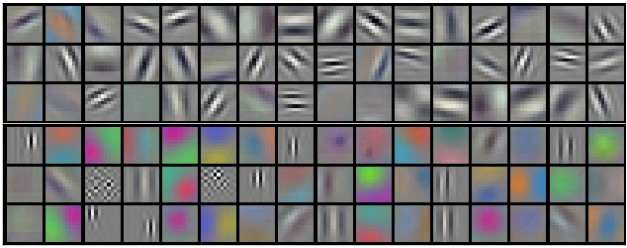
Overview and intuition without brain stuff. Lets first discuss what the CONV layer computes without brain/neuron analogies. The CONV layer’s parameters consist of a set of learnable filters. Every filter is small spatially (along width and height), but extends through the full depth of the input volume. For example, a typical filter on a first layer of a ConvNet might have size 5x5x3 (i.e. 5 pixels width and height, and 3 because images have depth 3, the color channels). During the forward pass, we slide (more precisely, convolve) each filter across the width and height of the input volume and compute dot products between the entries of the filter and the input at any position. As we slide the filter over the width and height of the input volume we will produce a 2-dimensional activation map that gives the responses of that filter at every spatial position. Intuitively, the network will learn filters that activate when they see some type of visual feature such as an edge of some orientation or a blotch of some color on the first layer, or eventually entire honeycomb or wheel-like patterns on higher layers of the network. Now, we will have an entire set of filters in each CONV layer (e.g. 12 filters), and each of them will produce a separate 2-dimensional activation map. We will stack these activation maps along the depth dimension and produce the output volume.

The brain view. If you’re a fan of the brain/neuron analogies, every entry in the 3D output volume can also be interpreted as an output of a neuron that looks at only a small region in the input and shares parameters with all neurons to the left and right spatially (since these numbers all result from applying the same filter). We now discuss the details of the neuron connectivities, their arrangement in space, and their parameter sharing scheme.

Local Connectivity. When dealing with high-dimensional inputs such as images, as we saw above it is impractical to connect neurons to all neurons in the previous volume. Instead, we will connect each neuron to only a local region of the input volume. The spatial extent of this connectivity is a hyperparameter called the receptive field of the neuron (equivalently this is the filter size). The extent of the connectivity along the depth axis is always equal to the depth of the input volume. It is important to emphasize again this asymmetry in how we treat the spatial dimensions (width and height) and the depth dimension: The connections are local in space (along width and height), but always full along the entire depth of the input volume.

Example 1. For example, suppose that the input volume has size [32x32x3], (e.g. an RGB CIFAR-10 image). If the receptive field (or the filter size) is 5x5, then each neuron in the Conv Layer will have weights to a [5x5x3] region in the input volume, for a total of 5*5*3 = 75 weights (and +1 bias parameter). Notice that the extent of the connectivity along the depth axis must be 3, since this is the depth of the input volume.

Example 2. Suppose an input volume had size [16x16x20]. Then using an example receptive field size of 3x3, every neuron in the Conv Layer would now have a total of 3*3*20 = 180 connections to the input volume. Notice that, again, the connectivity is local in space (e.g. 3x3), but full along the input depth (20).

Left: An example input volume in red (e.g. a 32x32x3 CIFAR-10 image), and an example volume of neurons in the first Convolutional layer. Each neuron in the convolutional layer is connected only to a local region in the input volume spatially, but to the full depth (i.e. all color channels). Note, there are multiple neurons (5 in this example) along the depth, all looking at the same region in the input - see discussion of depth columns in text below. Right: The neurons from the Neural Network chapter remain unchanged: They still compute a dot product of their weights with the input followed by a non-linearity, but their connectivity is now restricted to be local spatially.

Spatial arrangement. We have explained the connectivity of each neuron in the Conv Layer to the input volume, but we haven’t yet discussed how many neurons there are in the output volume or how they are arranged. Three hyperparameters control the size of the output volume: the depth, stride and zero-padding. We discuss these next:

1. First, the depth of the output volume is a hyperparameter: it corresponds to the number of filters we would like to use, each learning to look for something different in the input. For example, if the first Convolutional Layer takes as input the raw image, then different neurons along the depth dimension may activate in presence of various oriented edges, or blobs of color. We will refer to a set of neurons that are all looking at the same region of the input as a depth column (some people also prefer the term fibre).
2. Second, we must specify the stride with which we slide the filter. When the stride is 1 then we move the filters one pixel at a time. When the stride is 2 (or uncommonly 3 or more, though this is rare in practice) then the filters jump 2 pixels at a time as we slide them around. This will produce smaller output volumes spatially.
3. As we will soon see, sometimes it will be convenient to pad the input volume with zeros around the border. The size of this zero-padding is a hyperparameter. The nice feature of zero padding is that it will allow us to control the spatial size of the output volumes (most commonly as we’ll see soon we will use it to exactly preserve the spatial size of the input volume so the input and output width and height are the same).

We can compute the spatial size of the output volume as a function of the input volume size (W

), the receptive field size of the Conv Layer neurons ( F), the stride with which they are applied ( S), and the amount of zero padding used ( P) on the border. You can convince yourself that the correct formula for calculating how many neurons “fit” is given by (W−F+2P)/S+1

. For example for a 7x7 input and a 3x3 filter with stride 1 and pad 0 we would get a 5x5 output. With stride 2 we would get a 3x3 output. Lets also see one more graphical example:

Illustration of spatial arrangement. In this example there is only one spatial dimension (x-axis), one neuron with a receptive field size of F = 3, the input size is W = 5, and there is zero padding of P = 1. Left: The neuron strided across the input in stride of S = 1, giving output of size (5 - 3 + 2)/1+1 = 5. Right: The neuron uses stride of S = 2, giving output of size (5 - 3 + 2)/2+1 = 3. Notice that stride S = 3 could not be used since it wouldn't fit neatly across the volume. In terms of the equation, this can be determined since (5 - 3 + 2) = 4 is not divisible by 3.
The neuron weights are in this example [1,0,-1] (shown on very right), and its bias is zero. These weights are shared across all yellow neurons (see parameter sharing below).

Use of zero-padding. In the example above on left, note that the input dimension was 5 and the output dimension was equal: also 5. This worked out so because our receptive fields were 3 and we used zero padding of 1. If there was no zero-padding used, then the output volume would have had spatial dimension of only 3, because that it is how many neurons would have “fit” across the original input. In general, setting zero padding to be P=(F−1)/2

when the stride is S=1

ensures that the input volume and output volume will have the same size spatially. It is very common to use zero-padding in this way and we will discuss the full reasons when we talk more about ConvNet architectures.

Constraints on strides. Note again that the spatial arrangement hyperparameters have mutual constraints. For example, when the input has size W=10

, no zero-padding is used P=0, and the filter size is F=3, then it would be impossible to use stride S=2, since (W−F+2P)/S+1=(10−3+0)/2+1=4.5

, i.e. not an integer, indicating that the neurons don’t “fit” neatly and symmetrically across the input. Therefore, this setting of the hyperparameters is considered to be invalid, and a ConvNet library could throw an exception or zero pad the rest to make it fit, or crop the input to make it fit, or something. As we will see in the ConvNet architectures section, sizing the ConvNets appropriately so that all the dimensions “work out” can be a real headache, which the use of zero-padding and some design guidelines will significantly alleviate.

Real-world example. The Krizhevsky et al. architecture that won the ImageNet challenge in 2012 accepted images of size [227x227x3]. On the first Convolutional Layer, it used neurons with receptive field size F=11

, stride S=4 and no zero padding P=0. Since (227 - 11)/4 + 1 = 55, and since the Conv layer had a depth of K=96

, the Conv layer output volume had size [55x55x96]. Each of the 55*55*96 neurons in this volume was connected to a region of size [11x11x3] in the input volume. Moreover, all 96 neurons in each depth column are connected to the same [11x11x3] region of the input, but of course with different weights. As a fun aside, if you read the actual paper it claims that the input images were 224x224, which is surely incorrect because (224 - 11)/4 + 1 is quite clearly not an integer. This has confused many people in the history of ConvNets and little is known about what happened. My own best guess is that Alex used zero-padding of 3 extra pixels that he does not mention in the paper.

Parameter Sharing. Parameter sharing scheme is used in Convolutional Layers to control the number of parameters. Using the real-world example above, we see that there are 55*55*96 = 290,400 neurons in the first Conv Layer, and each has 11*11*3 = 363 weights and 1 bias. Together, this adds up to 290400 * 364 = 105,705,600 parameters on the first layer of the ConvNet alone. Clearly, this number is very high.

It turns out that we can dramatically reduce the number of parameters by making one reasonable assumption: That if one feature is useful to compute at some spatial position (x,y), then it should also be useful to compute at a different position (x2,y2). In other words, denoting a single 2-dimensional slice of depth as a depth slice (e.g. a volume of size [55x55x96] has 96 depth slices, each of size [55x55]), we are going to constrain the neurons in each depth slice to use the same weights and bias. With this parameter sharing scheme, the first Conv Layer in our example would now have only 96 unique set of weights (one for each depth slice), for a total of 96*11*11*3 = 34,848 unique weights, or 34,944 parameters (+96 biases). Alternatively, all 55*55 neurons in each depth slice will now be using the same parameters. In practice during backpropagation, every neuron in the volume will compute the gradient for its weights, but these gradients will be added up across each depth slice and only update a single set of weights per slice.

Notice that if all neurons in a single depth slice are using the same weight vector, then the forward pass of the CONV layer can in each depth slice be computed as a convolution of the neuron’s weights with the input volume (Hence the name: Convolutional Layer). This is why it is common to refer to the sets of weights as a filter (or a kernel), that is convolved with the input.

Example filters learned by Krizhevsky et al. Each of the 96 filters shown here is of size [11x11x3], and each one is shared by the 55*55 neurons in one depth slice. Notice that the parameter sharing assumption is relatively reasonable: If detecting a horizontal edge is important at some location in the image, it should intuitively be useful at some other location as well due to the translationally-invariant structure of images. There is therefore no need to relearn to detect a horizontal edge at every one of the 55*55 distinct locations in the Conv layer output volume.

Note that sometimes the parameter sharing assumption may not make sense. This is especially the case when the input images to a ConvNet have some specific centered structure, where we should expect, for example, that completely different features should be learned on one side of the image than another. One practical example is when the input are faces that have been centered in the image. You might expect that different eye-specific or hair-specific features could (and should) be learned in different spatial locations. In that case it is common to relax the parameter sharing scheme, and instead simply call the layer a Locally-Connected Layer.

Numpy examples. To make the discussion above more concrete, lets express the same ideas but in code and with a specific example. Suppose that the input volume is a numpy array X. Then:

• A depth column (or a fibre) at position (x,y) would be the activations X[x,y,:].
• A depth slice, or equivalently an activation map at depth d would be the activations X[:,:,d].

Conv Layer Example. Suppose that the input volume X has shape X.shape: (11,11,4). Suppose further that we use no zero padding (P=0

), that the filter size is F=5, and that the stride is S=2

. The output volume would therefore have spatial size (11-5)/2+1 = 4, giving a volume with width and height of 4. The activation map in the output volume (call it V), would then look as follows (only some of the elements are computed in this example):

• V[0,0,0] = np.sum(X[:5,:5,:] * W0) + b0
• V[1,0,0] = np.sum(X[2:7,:5,:] * W0) + b0
• V[2,0,0] = np.sum(X[4:9,:5,:] * W0) + b0
• V[3,0,0] = np.sum(X[6:11,:5,:] * W0) + b0

Remember that in numpy, the operation * above denotes elementwise multiplication between the arrays. Notice also that the weight vector W0 is the weight vector of that neuron and b0 is the bias. Here, W0 is assumed to be of shape W0.shape: (5,5,4), since the filter size is 5 and the depth of the input volume is 4. Notice that at each point, we are computing the dot product as seen before in ordinary neural networks. Also, we see that we are using the same weight and bias (due to parameter sharing), and where the dimensions along the width are increasing in steps of 2 (i.e. the stride). To construct a second activation map in the output volume, we would have:

• V[0,0,1] = np.sum(X[:5,:5,:] * W1) + b1
• V[1,0,1] = np.sum(X[2:7,:5,:] * W1) + b1
• V[2,0,1] = np.sum(X[4:9,:5,:] * W1) + b1
• V[3,0,1] = np.sum(X[6:11,:5,:] * W1) + b1
• V[0,1,1] = np.sum(X[:5,2:7,:] * W1) + b1 (example of going along y)
• V[2,3,1] = np.sum(X[4:9,6:11,:] * W1) + b1 (or along both)

where we see that we are indexing into the second depth dimension in V (at index 1) because we are computing the second activation map, and that a different set of parameters (W1) is now used. In the example above, we are for brevity leaving out some of the other operations the Conv Layer would perform to fill the other parts of the output array V. Additionally, recall that these activation maps are often followed elementwise through an activation function such as ReLU, but this is not shown here.

Summary. To summarize, the Conv Layer:

• Accepts a volume of size W1×H1×D1

Requires four hyperparameters:

• Number of filters K

, their spatial extent F, the stride S, the amount of zero padding P

• .

Produces a volume of size W2×H2×D2 where:

• W2=(W1−F+2P)/S+1

H2=(H1−F+2P)/S+1 (i.e. width and height are computed equally by symmetry) D2=K

• 
  

With parameter sharing, it introduces F⋅F⋅D1 weights per filter, for a total of (F⋅F⋅D1)⋅K weights and K biases. In the output volume, the d-th depth slice (of size W2×H2) is the result of performing a valid convolution of the d-th filter over the input volume with a stride of S, and then offset by d

• -th bias.

A common setting of the hyperparameters is F=3,S=1,P=1

. However, there are common conventions and rules of thumb that motivate these hyperparameters. See the ConvNet architectures section below.

Convolution Demo. Below is a running demo of a CONV layer. Since 3D volumes are hard to visualize, all the volumes (the input volume (in blue), the weight volumes (in red), the output volume (in green)) are visualized with each depth slice stacked in rows. The input volume is of size W1=5,H1=5,D1=3

, and the CONV layer parameters are K=2,F=3,S=2,P=1. That is, we have two filters of size 3×3, and they are applied with a stride of 2. Therefore, the output volume size has spatial size (5 - 3 + 2)/2 + 1 = 3. Moreover, notice that a padding of P=1

is applied to the input volume, making the outer border of the input volume zero. The visualization below iterates over the output activations (green), and shows that each element is computed by elementwise multiplying the highlighted input (blue) with the filter (red), summing it up, and then offsetting the result by the bias.

Implementation as Matrix Multiplication. Note that the convolution operation essentially performs dot products between the filters and local regions of the input. A common implementation pattern of the CONV layer is to take advantage of this fact and formulate the forward pass of a convolutional layer as one big matrix multiply as follows:

1. The local regions in the input image are stretched out into columns in an operation commonly called im2col. For example, if the input is [227x227x3] and it is to be convolved with 11x11x3 filters at stride 4, then we would take [11x11x3] blocks of pixels in the input and stretch each block into a column vector of size 11*11*3 = 363. Iterating this process in the input at stride of 4 gives (227-11)/4+1 = 55 locations along both width and height, leading to an output matrix X_col of im2col of size [363 x 3025], where every column is a stretched out receptive field and there are 55*55 = 3025 of them in total. Note that since the receptive fields overlap, every number in the input volume may be duplicated in multiple distinct columns.
2. The weights of the CONV layer are similarly stretched out into rows. For example, if there are 96 filters of size [11x11x3] this would give a matrix W_row of size [96 x 363].
3. The result of a convolution is now equivalent to performing one large matrix multiply np.dot(W_row, X_col), which evaluates the dot product between every filter and every receptive field location. In our example, the output of this operation would be [96 x 3025], giving the output of the dot product of each filter at each location.
4. The result must finally be reshaped back to its proper output dimension [55x55x96].

This approach has the downside that it can use a lot of memory, since some values in the input volume are replicated multiple times in X_col. However, the benefit is that there are many very efficient implementations of Matrix Multiplication that we can take advantage of (for example, in the commonly used BLAS API). Moreover, the same im2col idea can be reused to perform the pooling operation, which we discuss next.

Backpropagation. The backward pass for a convolution operation (for both the data and the weights) is also a convolution (but with spatially-flipped filters). This is easy to derive in the 1-dimensional case with a toy example (not expanded on for now).

1x1 convolution. As an aside, several papers use 1x1 convolutions, as first investigated by Network in Network. Some people are at first confused to see 1x1 convolutions especially when they come from signal processing background. Normally signals are 2-dimensional so 1x1 convolutions do not make sense (it’s just pointwise scaling). However, in ConvNets this is not the case because one must remember that we operate over 3-dimensional volumes, and that the filters always extend through the full depth of the input volume. For example, if the input is [32x32x3] then doing 1x1 convolutions would effectively be doing 3-dimensional dot products (since the input depth is 3 channels).

Dilated convolutions. A recent development (e.g. see paper by Fisher Yu and Vladlen Koltun) is to introduce one more hyperparameter to the CONV layer called the dilation. So far we’ve only discussed CONV filters that are contiguous. However, it’s possible to have filters that have spaces between each cell, called dilation. As an example, in one dimension a filter w of size 3 would compute over input x the following: w[0]*x[0] + w[1]*x[1] + w[2]*x[2]. This is dilation of 0. For dilation 1 the filter would instead compute w[0]*x[0] + w[1]*x[2] + w[2]*x[4]; In other words there is a gap of 1 between the applications. This can be very useful in some settings to use in conjunction with 0-dilated filters because it allows you to merge spatial information across the inputs much more agressively with fewer layers. For example, if you stack two 3x3 CONV layers on top of each other then you can convince yourself that the neurons on the 2nd layer are a function of a 5x5 patch of the input (we would say that the effective receptive field of these neurons is 5x5). If we use dilated convolutions then this effective receptive field would grow much quicker.

Pooling Layer

It is common to periodically insert a Pooling layer in-between successive Conv layers in a ConvNet architecture. Its function is to progressively reduce the spatial size of the representation to reduce the amount of parameters and computation in the network, and hence to also control overfitting. The Pooling Layer operates independently on every depth slice of the input and resizes it spatially, using the MAX operation. The most common form is a pooling layer with filters of size 2x2 applied with a stride of 2 downsamples every depth slice in the input by 2 along both width and height, discarding 75% of the activations. Every MAX operation would in this case be taking a max over 4 numbers (little 2x2 region in some depth slice). The depth dimension remains unchanged. More generally, the pooling layer:

• Accepts a volume of size W1×H1×D1

Requires two hyperparameters:

• their spatial extent F

, the stride S

• ,

Produces a volume of size W2×H2×D2 where:

• W2=(W1−F)/S+1

H2=(H1−F)/S+1
D2=D1

• • 
    
• Introduces zero parameters since it computes a fixed function of the input
• Note that it is not common to use zero-padding for Pooling layers

It is worth noting that there are only two commonly seen variations of the max pooling layer found in practice: A pooling layer with F=3,S=2

(also called overlapping pooling), and more commonly F=2,S=2

. Pooling sizes with larger receptive fields are too destructive.

General pooling. In addition to max pooling, the pooling units can also perform other functions, such as average pooling or even L2-norm pooling. Average pooling was often used historically but has recently fallen out of favor compared to the max pooling operation, which has been shown to work better in practice.

Pooling layer downsamples the volume spatially, independently in each depth slice of the input volume. Left: In this example, the input volume of size [224x224x64] is pooled with filter size 2, stride 2 into output volume of size [112x112x64]. Notice that the volume depth is preserved. Right: The most common downsampling operation is max, giving rise to max pooling, here shown with a stride of 2. That is, each max is taken over 4 numbers (little 2x2 square).

Backpropagation. Recall from the backpropagation chapter that the backward pass for a max(x, y) operation has a simple interpretation as only routing the gradient to the input that had the highest value in the forward pass. Hence, during the forward pass of a pooling layer it is common to keep track of the index of the max activation (sometimes also called the switches) so that gradient routing is efficient during backpropagation.

Getting rid of pooling. Many people dislike the pooling operation and think that we can get away without it. For example, Striving for Simplicity: The All Convolutional Net proposes to discard the pooling layer in favor of architecture that only consists of repeated CONV layers. To reduce the size of the representation they suggest using larger stride in CONV layer once in a while. Discarding pooling layers has also been found to be important in training good generative models, such as variational autoencoders (VAEs) or generative adversarial networks (GANs). It seems likely that future architectures will feature very few to no pooling layers.

Normalization Layer

Many types of normalization layers have been proposed for use in ConvNet architectures, sometimes with the intentions of implementing inhibition schemes observed in the biological brain. However, these layers have since fallen out of favor because in practice their contribution has been shown to be minimal, if any. For various types of normalizations, see the discussion in Alex Krizhevsky’s cuda-convnet library API.

Fully-connected layer

Neurons in a fully connected layer have full connections to all activations in the previous layer, as seen in regular Neural Networks. Their activations can hence be computed with a matrix multiplication followed by a bias offset. See the Neural Network section of the notes for more information.

Converting FC layers to CONV layers

It is worth noting that the only difference between FC and CONV layers is that the neurons in the CONV layer are connected only to a local region in the input, and that many of the neurons in a CONV volume share parameters. However, the neurons in both layers still compute dot products, so their functional form is identical. Therefore, it turns out that it’s possible to convert between FC and CONV layers:

• For any CONV layer there is an FC layer that implements the same forward function. The weight matrix would be a large matrix that is mostly zero except for at certain blocks (due to local connectivity) where the weights in many of the blocks are equal (due to parameter sharing).
• Conversely, any FC layer can be converted to a CONV layer. For example, an FC layer with K=4096

that is looking at some input volume of size 7×7×512 can be equivalently expressed as a CONV layer with F=7,P=0,S=1,K=4096. In other words, we are setting the filter size to be exactly the size of the input volume, and hence the output will simply be 1×1×4096

• since only a single depth column “fits” across the input volume, giving identical result as the initial FC layer.

FC->CONV conversion. Of these two conversions, the ability to convert an FC layer to a CONV layer is particularly useful in practice. Consider a ConvNet architecture that takes a 224x224x3 image, and then uses a series of CONV layers and POOL layers to reduce the image to an activations volume of size 7x7x512 (in an AlexNet architecture that we’ll see later, this is done by use of 5 pooling layers that downsample the input spatially by a factor of two each time, making the final spatial size 224/2/2/2/2/2 = 7). From there, an AlexNet uses two FC layers of size 4096 and finally the last FC layers with 1000 neurons that compute the class scores. We can convert each of these three FC layers to CONV layers as described above:

• Replace the first FC layer that looks at [7x7x512] volume with a CONV layer that uses filter size F=7

, giving output volume [1x1x4096]. Replace the second FC layer with a CONV layer that uses filter size F=1, giving output volume [1x1x4096] Replace the last FC layer similarly, with F=1

• , giving final output [1x1x1000]

Each of these conversions could in practice involve manipulating (e.g. reshaping) the weight matrix W

in each FC layer into CONV layer filters. It turns out that this conversion allows us to “slide” the original ConvNet very efficiently across many spatial positions in a larger image, in a single forward pass.

For example, if 224x224 image gives a volume of size [7x7x512] - i.e. a reduction by 32, then forwarding an image of size 384x384 through the converted architecture would give the equivalent volume in size [12x12x512], since 384/32 = 12. Following through with the next 3 CONV layers that we just converted from FC layers would now give the final volume of size [6x6x1000], since (12 - 7)/1 + 1 = 6. Note that instead of a single vector of class scores of size [1x1x1000], we’re now getting an entire 6x6 array of class scores across the 384x384 image.

Evaluating the original ConvNet (with FC layers) independently across 224x224 crops of the 384x384 image in strides of 32 pixels gives an identical result to forwarding the converted ConvNet one time.

Naturally, forwarding the converted ConvNet a single time is much more efficient than iterating the original ConvNet over all those 36 locations, since the 36 evaluations share computation. This trick is often used in practice to get better performance, where for example, it is common to resize an image to make it bigger, use a converted ConvNet to evaluate the class scores at many spatial positions and then average the class scores.

Lastly, what if we wanted to efficiently apply the original ConvNet over the image but at a stride smaller than 32 pixels? We could achieve this with multiple forward passes. For example, note that if we wanted to use a stride of 16 pixels we could do so by combining the volumes received by forwarding the converted ConvNet twice: First over the original image and second over the image but with the image shifted spatially by 16 pixels along both width and height.

• An IPython Notebook on Net Surgery shows how to perform the conversion in practice, in code (using Caffe)

ConvNet Architectures

We have seen that Convolutional Networks are commonly made up of only three layer types: CONV, POOL (we assume Max pool unless stated otherwise) and FC (short for fully-connected). We will also explicitly write the RELU activation function as a layer, which applies elementwise non-linearity. In this section we discuss how these are commonly stacked together to form entire ConvNets.

Layer Patterns

The most common form of a ConvNet architecture stacks a few CONV-RELU layers, follows them with POOL layers, and repeats this pattern until the image has been merged spatially to a small size. At some point, it is common to transition to fully-connected layers. The last fully-connected layer holds the output, such as the class scores. In other words, the most common ConvNet architecture follows the pattern:

INPUT -> [[CONV -> RELU]*N -> POOL?]*M -> [FC -> RELU]*K -> FC

where the * indicates repetition, and the POOL? indicates an optional pooling layer. Moreover, N >= 0 (and usually N <= 3), M >= 0, K >= 0 (and usually K < 3). For example, here are some common ConvNet architectures you may see that follow this pattern:

• INPUT -> FC, implements a linear classifier. Here N = M = K = 0.
• INPUT -> CONV -> RELU -> FC
• INPUT -> [CONV -> RELU -> POOL]*2 -> FC -> RELU -> FC. Here we see that there is a single CONV layer between every POOL layer.
• INPUT -> [CONV -> RELU -> CONV -> RELU -> POOL]*3 -> [FC -> RELU]*2 -> FC Here we see two CONV layers stacked before every POOL layer. This is generally a good idea for larger and deeper networks, because multiple stacked CONV layers can develop more complex features of the input volume before the destructive pooling operation.

Prefer a stack of small filter CONV to one large receptive field CONV layer. Suppose that you stack three 3x3 CONV layers on top of each other (with non-linearities in between, of course). In this arrangement, each neuron on the first CONV layer has a 3x3 view of the input volume. A neuron on the second CONV layer has a 3x3 view of the first CONV layer, and hence by extension a 5x5 view of the input volume. Similarly, a neuron on the third CONV layer has a 3x3 view of the 2nd CONV layer, and hence a 7x7 view of the input volume. Suppose that instead of these three layers of 3x3 CONV, we only wanted to use a single CONV layer with 7x7 receptive fields. These neurons would have a receptive field size of the input volume that is identical in spatial extent (7x7), but with several disadvantages. First, the neurons would be computing a linear function over the input, while the three stacks of CONV layers contain non-linearities that make their features more expressive. Second, if we suppose that all the volumes have C

channels, then it can be seen that the single 7x7 CONV layer would contain C×(7×7×C)=49C2 parameters, while the three 3x3 CONV layers would only contain 3×(C×(3×3×C))=27C2

parameters. Intuitively, stacking CONV layers with tiny filters as opposed to having one CONV layer with big filters allows us to express more powerful features of the input, and with fewer parameters. As a practical disadvantage, we might need more memory to hold all the intermediate CONV layer results if we plan to do backpropagation.

Recent departures. It should be noted that the conventional paradigm of a linear list of layers has recently been challenged, in Google’s Inception architectures and also in current (state of the art) Residual Networks from Microsoft Research Asia. Both of these (see details below in case studies section) feature more intricate and different connectivity structures.

In practice: use whatever works best on ImageNet. If you’re feeling a bit of a fatigue in thinking about the architectural decisions, you’ll be pleased to know that in 90% or more of applications you should not have to worry about these. I like to summarize this point as “don’t be a hero”: Instead of rolling your own architecture for a problem, you should look at whatever architecture currently works best on ImageNet, download a pretrained model and finetune it on your data. You should rarely ever have to train a ConvNet from scratch or design one from scratch. I also made this point at the Deep Learning school.

Layer Sizing Patterns

Until now we’ve omitted mentions of common hyperparameters used in each of the layers in a ConvNet. We will first state the common rules of thumb for sizing the architectures and then follow the rules with a discussion of the notation:

The input layer (that contains the image) should be divisible by 2 many times. Common numbers include 32 (e.g. CIFAR-10), 64, 96 (e.g. STL-10), or 224 (e.g. common ImageNet ConvNets), 384, and 512.

The conv layers should be using small filters (e.g. 3x3 or at most 5x5), using a stride of S=1

, and crucially, padding the input volume with zeros in such way that the conv layer does not alter the spatial dimensions of the input. That is, when F=3, then using P=1 will retain the original size of the input. When F=5, P=2. For a general F, it can be seen that P=(F−1)/2

preserves the input size. If you must use bigger filter sizes (such as 7x7 or so), it is only common to see this on the very first conv layer that is looking at the input image.

The pool layers are in charge of downsampling the spatial dimensions of the input. The most common setting is to use max-pooling with 2x2 receptive fields (i.e. F=2

), and with a stride of 2 (i.e. S=2

). Note that this discards exactly 75% of the activations in an input volume (due to downsampling by 2 in both width and height). Another slightly less common setting is to use 3x3 receptive fields with a stride of 2, but this makes. It is very uncommon to see receptive field sizes for max pooling that are larger than 3 because the pooling is then too lossy and aggressive. This usually leads to worse performance.

Reducing sizing headaches. The scheme presented above is pleasing because all the CONV layers preserve the spatial size of their input, while the POOL layers alone are in charge of down-sampling the volumes spatially. In an alternative scheme where we use strides greater than 1 or don’t zero-pad the input in CONV layers, we would have to very carefully keep track of the input volumes throughout the CNN architecture and make sure that all strides and filters “work out”, and that the ConvNet architecture is nicely and symmetrically wired.

Why use stride of 1 in CONV? Smaller strides work better in practice. Additionally, as already mentioned stride 1 allows us to leave all spatial down-sampling to the POOL layers, with the CONV layers only transforming the input volume depth-wise.

Why use padding? In addition to the aforementioned benefit of keeping the spatial sizes constant after CONV, doing this actually improves performance. If the CONV layers were to not zero-pad the inputs and only perform valid convolutions, then the size of the volumes would reduce by a small amount after each CONV, and the information at the borders would be “washed away” too quickly.

Compromising based on memory constraints. In some cases (especially early in the ConvNet architectures), the amount of memory can build up very quickly with the rules of thumb presented above. For example, filtering a 224x224x3 image with three 3x3 CONV layers with 64 filters each and padding 1 would create three activation volumes of size [224x224x64]. This amounts to a total of about 10 million activations, or 72MB of memory (per image, for both activations and gradients). Since GPUs are often bottlenecked by memory, it may be necessary to compromise. In practice, people prefer to make the compromise at only the first CONV layer of the network. For example, one compromise might be to use a first CONV layer with filter sizes of 7x7 and stride of 2 (as seen in a ZF net). As another example, an AlexNet uses filter sizes of 11x11 and stride of 4.

Case studies

There are several architectures in the field of Convolutional Networks that have a name. The most common are:

• LeNet. The first successful applications of Convolutional Networks were developed by Yann LeCun in 1990’s. Of these, the best known is the LeNet architecture that was used to read zip codes, digits, etc.
• AlexNet. The first work that popularized Convolutional Networks in Computer Vision was the AlexNet, developed by Alex Krizhevsky, Ilya Sutskever and Geoff Hinton. The AlexNet was submitted to the ImageNet ILSVRC challenge in 2012 and significantly outperformed the second runner-up (top 5 error of 16% compared to runner-up with 26% error). The Network had a very similar architecture to LeNet, but was deeper, bigger, and featured Convolutional Layers stacked on top of each other (previously it was common to only have a single CONV layer always immediately followed by a POOL layer).
• ZF Net. The ILSVRC 2013 winner was a Convolutional Network from Matthew Zeiler and Rob Fergus. It became known as the ZFNet (short for Zeiler & Fergus Net). It was an improvement on AlexNet by tweaking the architecture hyperparameters, in particular by expanding the size of the middle convolutional layers and making the stride and filter size on the first layer smaller.
• GoogLeNet. The ILSVRC 2014 winner was a Convolutional Network from Szegedy et al. from Google. Its main contribution was the development of an Inception Module that dramatically reduced the number of parameters in the network (4M, compared to AlexNet with 60M). Additionally, this paper uses Average Pooling instead of Fully Connected layers at the top of the ConvNet, eliminating a large amount of parameters that do not seem to matter much. There are also several followup versions to the GoogLeNet, most recently Inception-v4.
• VGGNet. The runner-up in ILSVRC 2014 was the network from Karen Simonyan and Andrew Zisserman that became known as the VGGNet. Its main contribution was in showing that the depth of the network is a critical component for good performance. Their final best network contains 16 CONV/FC layers and, appealingly, features an extremely homogeneous architecture that only performs 3x3 convolutions and 2x2 pooling from the beginning to the end. Their pretrained model is available for plug and play use in Caffe. A downside of the VGGNet is that it is more expensive to evaluate and uses a lot more memory and parameters (140M). Most of these parameters are in the first fully connected layer, and it was since found that these FC layers can be removed with no performance downgrade, significantly reducing the number of necessary parameters.
• ResNet. Residual Network developed by Kaiming He et al. was the winner of ILSVRC 2015. It features special skip connections and a heavy use of batch normalization. The architecture is also missing fully connected layers at the end of the network. The reader is also referred to Kaiming’s presentation (video, slides), and some recent experiments that reproduce these networks in Torch. ResNets are currently by far state of the art Convolutional Neural Network models and are the default choice for using ConvNets in practice (as of May 10, 2016). In particular, also see more recent developments that tweak the original architecture from Kaiming He et al. Identity Mappings in Deep Residual Networks (published March 2016).

VGGNet in detail.Lets break down the VGGNet in more detail as a case study. The whole VGGNet is composed of CONV layers that perform 3x3 convolutions with stride 1 and pad 1, and of POOL layers that perform 2x2 max pooling with stride 2 (and no padding). We can write out the size of the representation at each step of the processing and keep track of both the representation size and the total number of weights:

INPUT: [224x224x3]        memory:  224*224*3=150K   weights: 0
CONV3-64: [224x224x64]  memory:  224*224*64=3.2M   weights: (3*3*3)*64 = 1,728
CONV3-64: [224x224x64]  memory:  224*224*64=3.2M   weights: (3*3*64)*64 = 36,864
POOL2: [112x112x64]  memory:  112*112*64=800K   weights: 0
CONV3-128: [112x112x128]  memory:  112*112*128=1.6M   weights: (3*3*64)*128 = 73,728
CONV3-128: [112x112x128]  memory:  112*112*128=1.6M   weights: (3*3*128)*128 = 147,456
POOL2: [56x56x128]  memory:  56*56*128=400K   weights: 0
CONV3-256: [56x56x256]  memory:  56*56*256=800K   weights: (3*3*128)*256 = 294,912
CONV3-256: [56x56x256]  memory:  56*56*256=800K   weights: (3*3*256)*256 = 589,824
CONV3-256: [56x56x256]  memory:  56*56*256=800K   weights: (3*3*256)*256 = 589,824
POOL2: [28x28x256]  memory:  28*28*256=200K   weights: 0
CONV3-512: [28x28x512]  memory:  28*28*512=400K   weights: (3*3*256)*512 = 1,179,648
CONV3-512: [28x28x512]  memory:  28*28*512=400K   weights: (3*3*512)*512 = 2,359,296
CONV3-512: [28x28x512]  memory:  28*28*512=400K   weights: (3*3*512)*512 = 2,359,296
POOL2: [14x14x512]  memory:  14*14*512=100K   weights: 0
CONV3-512: [14x14x512]  memory:  14*14*512=100K   weights: (3*3*512)*512 = 2,359,296
CONV3-512: [14x14x512]  memory:  14*14*512=100K   weights: (3*3*512)*512 = 2,359,296
CONV3-512: [14x14x512]  memory:  14*14*512=100K   weights: (3*3*512)*512 = 2,359,296
POOL2: [7x7x512]  memory:  7*7*512=25K  weights: 0
FC: [1x1x4096]  memory:  4096  weights: 7*7*512*4096 = 102,760,448
FC: [1x1x4096]  memory:  4096  weights: 4096*4096 = 16,777,216
FC: [1x1x1000]  memory:  1000 weights: 4096*1000 = 4,096,000

TOTAL memory: 24M * 4 bytes ~= 93MB / image (only forward! ~*2 for bwd)
TOTAL params: 138M parameters

As is common with Convolutional Networks, notice that most of the memory (and also compute time) is used in the early CONV layers, and that most of the parameters are in the last FC layers. In this particular case, the first FC layer contains 100M weights, out of a total of 140M.

Computational Considerations

The largest bottleneck to be aware of when constructing ConvNet architectures is the memory bottleneck. Many modern GPUs have a limit of 3/4/6GB memory, with the best GPUs having about 12GB of memory. There are three major sources of memory to keep track of:

• From the intermediate volume sizes: These are the raw number of activations at every layer of the ConvNet, and also their gradients (of equal size). Usually, most of the activations are on the earlier layers of a ConvNet (i.e. first Conv Layers). These are kept around because they are needed for backpropagation, but a clever implementation that runs a ConvNet only at test time could in principle reduce this by a huge amount, by only storing the current activations at any layer and discarding the previous activations on layers below.
• From the parameter sizes: These are the numbers that hold the network parameters, their gradients during backpropagation, and commonly also a step cache if the optimization is using momentum, Adagrad, or RMSProp. Therefore, the memory to store the parameter vector alone must usually be multiplied by a factor of at least 3 or so.
• Every ConvNet implementation has to maintain miscellaneous memory, such as the image data batches, perhaps their augmented versions, etc.

Once you have a rough estimate of the total number of values (for activations, gradients, and misc), the number should be converted to size in GB. Take the number of values, multiply by 4 to get the raw number of bytes (since every floating point is 4 bytes, or maybe by 8 for double precision), and then divide by 1024 multiple times to get the amount of memory in KB, MB, and finally GB. If your network doesn’t fit, a common heuristic to “make it fit” is to decrease the batch size, since most of the memory is usually consumed by the activations.

Additional Resources

Additional resources related to implementation:

• Soumith benchmarks for CONV performance
• ConvNetJS CIFAR-10 demo allows you to play with ConvNet architectures and see the results and computations in real time, in the browser.
• Caffe, one of the popular ConvNet libraries.
• State of the art ResNets in Torch7