An easy way
使用torch.nn.Sequential()来更快地构建神经网络:
import torch
import torch.nn.functional as F


# replace following class code with an easy sequential network
class Net(torch.nn.Module):
    def __init__(self, n_feature, n_hidden, n_output):
        super(Net, self).__init__()
        self.hidden = torch.nn.Linear(n_feature, n_hidden)   # hidden layer
        self.predict = torch.nn.Linear(n_hidden, n_output)   # output layer

    def forward(self, x):
        x = F.relu(self.hidden(x))      # activation function for hidden layer
        x = self.predict(x)             # linear output
        return x

net1 = Net(1, 10, 1)

# easy and fast way to build your network
net2 = torch.nn.Sequential(
    torch.nn.Linear(1, 10),
    torch.nn.ReLU(),
    torch.nn.Linear(10, 1)
)


print(net1)     # net1 architecture
"""
Net (
  (hidden): Linear (1 -> 10)
  (predict): Linear (10 -> 1)
)
"""

print(net2)     # net2 architecture
"""
Sequential (
  (0): Linear (1 -> 10)
  (1): ReLU ()
  (2): Linear (10 -> 1)
)
"""
Save and reload
两种保存网络模型的方法:
torch.save(net1, 'net.pkl')  # save entire net
torch.save(net1.state_dict(), 'net_params.pkl')   # save only the parameters
读取模型:
net2 = torch.load('net.pkl')
prediction = net2(x)
只读取模型参数:
# restore only the parameters in net1 to net3
net3 = torch.nn.Sequential(
    torch.nn.Linear(1, 10),
    torch.nn.ReLU(),
    torch.nn.Linear(10, 1)
)

# copy net1's parameters into net3
net3.load_state_dict(torch.load('net_params.pkl'))
prediction = net3(x)
Train on batch
通过Data.DataLoader()中的batch_size参数来控制加载数据时的batch大小
import torch
import torch.utils.data as Data

torch.manual_seed(1)    # reproducible

BATCH_SIZE = 5
# BATCH_SIZE = 8

x = torch.linspace(1, 10, 10)       # this is x data (torch tensor)
y = torch.linspace(10, 1, 10)       # this is y data (torch tensor)

torch_dataset = Data.TensorDataset(x, y)
loader = Data.DataLoader(
    dataset=torch_dataset,      # torch TensorDataset format
    batch_size=BATCH_SIZE,      # mini batch size
    shuffle=True,               # random shuffle for training
    num_workers=2,              # subprocesses for loading data
)


def show_batch():
    for epoch in range(3):   # train entire dataset 3 times
        for step, (batch_x, batch_y) in enumerate(loader):  # for each training step
            # train your data...
            print('Epoch: ', epoch, '| Step: ', step, '| batch x: ',
                  batch_x.numpy(), '| batch y: ', batch_y.numpy())


if __name__ == '__main__':
    show_batch()
打印结果:
Epoch:  0 | Step:  0 | batch x:  [ 5.  7. 10.  3.  4.] | batch y:  [6. 4. 1. 8. 7.]
Epoch:  0 | Step:  1 | batch x:  [2. 1. 8. 9. 6.] | batch y:  [ 9. 10.  3.  2.  5.]
Epoch:  1 | Step:  0 | batch x:  [ 4.  6.  7. 10.  8.] | batch y:  [7. 5. 4. 1. 3.]
Epoch:  1 | Step:  1 | batch x:  [5. 3. 2. 1. 9.] | batch y:  [ 6.  8.  9. 10.  2.]
Epoch:  2 | Step:  0 | batch x:  [ 4.  2.  5.  6. 10.] | batch y:  [7. 9. 6. 5. 1.]
Epoch:  2 | Step:  1 | batch x:  [3. 9. 1. 8. 7.] | batch y:  [ 8.  2. 10.  3.  4.]
Optimizers
比较不同的优化方法对网络的影响:
import torch
import torch.utils.data as Data
import torch.nn.functional as F
import matplotlib.pyplot as plt

# torch.manual_seed(1)    # reproducible

LR = 0.01
BATCH_SIZE = 32
EPOCH = 12

# fake dataset
x = torch.unsqueeze(torch.linspace(-1, 1, 1000), dim=1)
y = x.pow(2) + 0.1*torch.normal(torch.zeros(*x.size()))

# plot dataset
plt.scatter(x.numpy(), y.numpy())
plt.show()

# put dateset into torch dataset
torch_dataset = Data.TensorDataset(x, y)
loader = Data.DataLoader(dataset=torch_dataset, batch_size=BATCH_SIZE, shuffle=True, num_workers=2,)


# default network
class Net(torch.nn.Module):
    def __init__(self):
        super(Net, self).__init__()
        self.hidden = torch.nn.Linear(1, 20)   # hidden layer
        self.predict = torch.nn.Linear(20, 1)   # output layer

    def forward(self, x):
        x = F.relu(self.hidden(x))      # activation function for hidden layer
        x = self.predict(x)             # linear output
        return x

if __name__ == '__main__':
    # different nets
    net_SGD         = Net()
    net_Momentum    = Net()
    net_RMSprop     = Net()
    net_Adam        = Net()
    nets = [net_SGD, net_Momentum, net_RMSprop, net_Adam]

    # different optimizers
    opt_SGD         = torch.optim.SGD(net_SGD.parameters(), lr=LR)
    opt_Momentum    = torch.optim.SGD(net_Momentum.parameters(), lr=LR, momentum=0.8)
    opt_RMSprop     = torch.optim.RMSprop(net_RMSprop.parameters(), lr=LR, alpha=0.9)
    opt_Adam        = torch.optim.Adam(net_Adam.parameters(), lr=LR, betas=(0.9, 0.99))
    optimizers = [opt_SGD, opt_Momentum, opt_RMSprop, opt_Adam]

    loss_func = torch.nn.MSELoss()
    losses_his = [[], [], [], []]   # record loss

    # training
    for epoch in range(EPOCH):
        print('Epoch: ', epoch)
        for step, (b_x, b_y) in enumerate(loader):          # for each training step
            for net, opt, l_his in zip(nets, optimizers, losses_his):
                output = net(b_x)              # get output for every net
                loss = loss_func(output, b_y)  # compute loss for every net
                opt.zero_grad()                # clear gradients for next train
                loss.backward()                # backpropagation, compute gradients
                opt.step()                     # apply gradients
                l_his.append(loss.data.numpy())     # loss recoder

    labels = ['SGD', 'Momentum', 'RMSprop', 'Adam']
    for i, l_his in enumerate(losses_his):
        plt.plot(l_his, label=labels[i])
    plt.legend(loc='best')
    plt.xlabel('Steps')
    plt.ylabel('Loss')
    plt.ylim((0, 0.2))
    plt.show()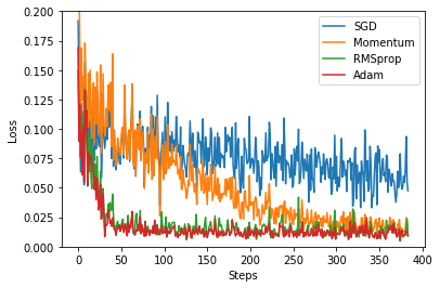
CNN
# library
# standard library
import os

# third-party library
import torch
import torch.nn as nn
import torch.utils.data as Data
import torchvision
import matplotlib.pyplot as plt

# torch.manual_seed(1)    # reproducible

# Hyper Parameters
EPOCH = 1               # train the training data n times, to save time, we just train 1 epoch
BATCH_SIZE = 50
LR = 0.001              # learning rate
DOWNLOAD_MNIST = False


# Mnist digits dataset
if not(os.path.exists('./mnist/')) or not os.listdir('./mnist/'):
    # not mnist dir or mnist is empyt dir
    DOWNLOAD_MNIST = True

train_data = torchvision.datasets.MNIST(
    root='./mnist/',
    train=True,                                     # this is training data
    transform=torchvision.transforms.ToTensor(),    # Converts a PIL.Image or numpy.ndarray to
                                                    # torch.FloatTensor of shape (C x H x W) and normalize in the range [0.0, 1.0]
    download=DOWNLOAD_MNIST,
)

# plot one example
print(train_data.train_data.size())                 # (60000, 28, 28)
print(train_data.train_labels.size())               # (60000)
plt.imshow(train_data.train_data[0].numpy(), cmap='gray')
plt.title('%i' % train_data.train_labels[0])
plt.show()

# Data Loader for easy mini-batch return in training, the image batch shape will be (50, 1, 28, 28)
train_loader = Data.DataLoader(dataset=train_data, batch_size=BATCH_SIZE, shuffle=True)

# pick 2000 samples to speed up testing
test_data = torchvision.datasets.MNIST(root='./mnist/', train=False)
test_x = torch.unsqueeze(test_data.test_data, dim=1).type(torch.FloatTensor)[:2000]/255.   # shape from (2000, 28, 28) to (2000, 1, 28, 28), value in range(0,1)
test_y = test_data.test_labels[:2000]


class CNN(nn.Module):
    def __init__(self):
        super(CNN, self).__init__()
        self.conv1 = nn.Sequential(         # input shape (1, 28, 28)
            nn.Conv2d(
                in_channels=1,              # input height
                out_channels=16,            # n_filters
                kernel_size=5,              # filter size
                stride=1,                   # filter movement/step
                padding=2,                  # if want same width and length of this image after Conv2d, padding=(kernel_size-1)/2 if stride=1
            ),                              # output shape (16, 28, 28)
            nn.ReLU(),                      # activation
            nn.MaxPool2d(kernel_size=2),    # choose max value in 2x2 area, output shape (16, 14, 14)
        )
        self.conv2 = nn.Sequential(         # input shape (16, 14, 14)
            nn.Conv2d(16, 32, 5, 1, 2),     # output shape (32, 14, 14)
            nn.ReLU(),                      # activation
            nn.MaxPool2d(2),                # output shape (32, 7, 7)
        )
        self.out = nn.Linear(32 * 7 * 7, 10)   # fully connected layer, output 10 classes

    def forward(self, x):
        x = self.conv1(x)
        x = self.conv2(x)
        x = x.view(x.size(0), -1)           # flatten the output of conv2 to (batch_size, 32 * 7 * 7)
        output = self.out(x)
        return output, x    # return x for visualization


cnn = CNN()
print(cnn)  # net architecture

optimizer = torch.optim.Adam(cnn.parameters(), lr=LR)   # optimize all cnn parameters
loss_func = nn.CrossEntropyLoss()                       # the target label is not one-hotted

# following function (plot_with_labels) is for visualization, can be ignored if not interested
from matplotlib import cm
try: from sklearn.manifold import TSNE; HAS_SK = True
except: HAS_SK = False; print('Please install sklearn for layer visualization')
def plot_with_labels(lowDWeights, labels):
    plt.cla()
    X, Y = lowDWeights[:, 0], lowDWeights[:, 1]
    for x, y, s in zip(X, Y, labels):
        c = cm.rainbow(int(255 * s / 9)); plt.text(x, y, s, backgroundcolor=c, fontsize=9)
    plt.xlim(X.min(), X.max()); plt.ylim(Y.min(), Y.max()); plt.title('Visualize last layer'); plt.show(); plt.pause(0.01)

plt.ion()
# training and testing
for epoch in range(EPOCH):
    for step, (b_x, b_y) in enumerate(train_loader):   # gives batch data, normalize x when iterate train_loader

        output = cnn(b_x)[0]               # cnn output
        loss = loss_func(output, b_y)   # cross entropy loss
        optimizer.zero_grad()           # clear gradients for this training step
        loss.backward()                 # backpropagation, compute gradients
        optimizer.step()                # apply gradients

        if step % 50 == 0:
            test_output, last_layer = cnn(test_x)
            pred_y = torch.max(test_output, 1)[1].data.numpy()
            accuracy = float((pred_y == test_y.data.numpy()).astype(int).sum()) / float(test_y.size(0))
            print('Epoch: ', epoch, '| train loss: %.4f' % loss.data.numpy(), '| test accuracy: %.2f' % accuracy)
            if HAS_SK:
                # Visualization of trained flatten layer (T-SNE)
                tsne = TSNE(perplexity=30, n_components=2, init='pca', n_iter=5000)
                plot_only = 500
                low_dim_embs = tsne.fit_transform(last_layer.data.numpy()[:plot_only, :])
                labels = test_y.numpy()[:plot_only]
                plot_with_labels(low_dim_embs, labels)
plt.ioff()

# print 10 predictions from test data
test_output, _ = cnn(test_x[:10])
pred_y = torch.max(test_output, 1)[1].data.numpy()
print(pred_y, 'prediction number')
print(test_y[:10].numpy(), 'real number')
参考: