前言
最近打算重新跟着官方教程学习一下caffe,顺便也自己翻译了一下官方的文档。自己也做了一些标注,都用斜体标记出来了。中间可能额外还加了自己遇到的问题或是运行结果之类的。欢迎交流指正,拒绝喷子!
官方教程的原文链接:http://nbviewer.jupyter.org/github/BVLC/caffe/blob/master/examples/01-learning-lenet.ipynb
Solving in Python with LeNet
在这个例子中我们将要学习Caffe的Python接口,着重学习Solver接口。
1.准备
- 准备好Python环境:我们通过使用
pylab库来导入numpy并绘图。
from pylab import *
%matplotlib inline- 导入
caffe,添加它的路径到sys.path。请事先编译好pycaffe。
import sys
caffe_root = '/home/xhb/caffe/caffe/' # caffe的根路径,请自行设置
sys.path.insert(0, caffe_root + 'python')
import caffe- 我们首先使用提供的LeNet例子的数据和网络模型(你需要自行下载好数据,并创建好数据库,如下所示)
# run scripts from caffe root
import os
os.chdir(caffe_root)
# Download data
!data/mnist/get_mnist.sh
# Prepare data
!examples/mnist/create_mnist.sh
# back to examples
os.chdir('examples')
Downloading...
Creating lmdb...
I0301 12:48:30.756855 995 db_lmdb.cpp:35] Opened lmdb examples/mnist/mnist_train_lmdb
I0301 12:48:30.757007 995 convert_mnist_data.cpp:88] A total of 60000 items.
I0301 12:48:30.757015 995 convert_mnist_data.cpp:89] Rows: 28 Cols: 28
I0301 12:48:35.242076 995 convert_mnist_data.cpp:108] Processed 60000 files.
I0301 12:48:35.257020 996 db_lmdb.cpp:35] Opened lmdb examples/mnist/mnist_test_lmdb
I0301 12:48:35.257267 996 convert_mnist_data.cpp:88] A total of 10000 items.
I0301 12:48:35.257280 996 convert_mnist_data.cpp:89] Rows: 28 Cols: 28
I0301 12:48:35.941156 996 convert_mnist_data.cpp:108] Processed 10000 files.
Done.
2.创建网络
现在让我们来编写一个LeNet的变种网络,经典的1989年的convnet结构。
我们另外需要两个文件:
- 网络的prototxt文件,定义了网络结构,并指向了训练和测试数据集。
- 解决方案的prototxt文件,定义了超参数等。
我们首先创建网络。我们将使用Python代码以简洁而自然的方式来编写网络,并序列化为Caffe的protobuf模型格式。
这个网络需要从生成好的LMDB数据库文件读取数据,单也可以使用MemoryDataLayer直接从ndarray读取数据。
from caffe import layers as L, params as P

def lenet(lmdb, batch_size):
    # our version of LeNet: a series of linear and simple nonlinear transformations
    n = caffe.NetSpec()

    n.data, n.label = L.Data(batch_size=batch_size, backend=P.Data.LMDB, source=lmdb,
                             transform_param=dict(scale=1./255), ntop=2)

    n.conv1 = L.Convolution(n.data, kernel_size=5, num_output=20, weight_filler=dict(type='xavier'))
    n.pool1 = L.Pooling(n.conv1, kernel_size=2, stride=2, pool=P.Pooling.MAX)
    n.conv2 = L.Convolution(n.pool1, kernel_size=5, num_output=50, weight_filler=dict(type='xavier'))
    n.pool2 = L.Pooling(n.conv2, kernel_size=2, stride=2, pool=P.Pooling.MAX)
    n.fc1 =   L.InnerProduct(n.pool2, num_output=500, weight_filler=dict(type='xavier'))
    n.relu1 = L.ReLU(n.fc1, in_place=True)
    n.score = L.InnerProduct(n.relu1, num_output=10, weight_filler=dict(type='xavier'))
    n.loss =  L.SoftmaxWithLoss(n.score, n.label)

    return n.to_proto()

with open('mnist/lenet_auto_train.prototxt', 'w') as f:
    f.write(str(lenet('mnist/mnist_train_lmdb', 64)))

with open('mnist/lenet_auto_test.prototxt', 'w') as f:
    f.write(str(lenet('mnist/mnist_test_lmdb', 100)))
通过使用Google的protobuf库,这个网络已经被以一种更加冗长单却易读的序列化格式保存到硬盘上了。你可以直接读取,写入,修改数据。让我们看看要训练的网络。
!cat mnist/lenet_auto_train.prototxtlayer {
name: "data"
type: "Data"
top: "data"
top: "label"
transform_param {
scale: 0.00392156885937
}
data_param {
source: "mnist/mnist_train_lmdb"
batch_size: 64
backend: LMDB
}
}
layer {
name: "conv1"
type: "Convolution"
bottom: "data"
top: "conv1"
convolution_param {
num_output: 20
kernel_size: 5
weight_filler {
type: "xavier"
}
}
}
layer {
name: "pool1"
type: "Pooling"
bottom: "conv1"
top: "pool1"
pooling_param {
pool: MAX
kernel_size: 2
stride: 2
}
}
layer {
name: "conv2"
type: "Convolution"
bottom: "pool1"
top: "conv2"
convolution_param {
num_output: 50
kernel_size: 5
weight_filler {
type: "xavier"
}
}
}
layer {
name: "pool2"
type: "Pooling"
bottom: "conv2"
top: "pool2"
pooling_param {
pool: MAX
kernel_size: 2
stride: 2
}
}
layer {
name: "fc1"
type: "InnerProduct"
bottom: "pool2"
top: "fc1"
inner_product_param {
num_output: 500
weight_filler {
type: "xavier"
}
}
}
layer {
name: "relu1"
type: "ReLU"
bottom: "fc1"
top: "fc1"
}
layer {
name: "score"
type: "InnerProduct"
bottom: "fc1"
top: "score"
inner_product_param {
num_output: 10
weight_filler {
type: "xavier"
}
}
}
layer {
name: "loss"
type: "SoftmaxWithLoss"
bottom: "score"
bottom: "label"
top: "loss"
}
现在让我们看看学习参数(超参数),它们都被保存在一个prototxt文件中(caffe源码中已经提供了)。我们使用有动量、权重衰减、指定的学习率表的SGD算法。
# 备注:这里我修改了lenet_auto_solver.prototxt,因为我不是在caffe_root下操作的,所以不能使用相关路径;
# 如果这个文件中的路径错了,后面的程序会直接死掉,无法运行,所以无法运行时可以查看下这个文件中定义的路径是否出错了
!cat mnist/lenet_auto_solver.prototxt
# The train/test net protocol buffer definition
# train_net: "mnist/lenet_auto_train.prototxt"
train_net: "/home/xhb/caffe/caffe/examples/mnist/lenet_auto_train.prototxt"
# test_net: "mnist/lenet_auto_test.prototxt"
test_net: "/home/xhb/caffe/caffe/examples/mnist/lenet_auto_test.prototxt"
# test_iter specifies how many forward passes the test should carry out.
# In the case of MNIST, we have test batch size 100 and 100 test iterations,
# covering the full 10,000 testing images.
test_iter: 100
# Carry out testing every 500 training iterations.
test_interval: 500
# The base learning rate, momentum and the weight decay of the network.
base_lr: 0.01
momentum: 0.9
weight_decay: 0.0005
# The learning rate policy
lr_policy: "inv"
gamma: 0.0001
power: 0.75
# Display every 100 iterations
display: 100
# The maximum number of iterations
max_iter: 10000
# snapshot intermediate results
snapshot: 5000
snapshot_prefix: "/home/xhb/caffe/caffe/examples/mnist/lenet"
3.导入并检验解决方案
- 我们选择一个设备,并导入解决方案(solver)。使用SGD算法(带动量)进行优化,但是其他优化算法也是可行的,比如Adagrad和Nesterov的加速梯度下降算法。
# 备注:我在笔记本上跑的,所以没有采用GPU模式,而是使用了CPU模式
# caffe.set_device(0)
# caffe.set_mode_gpu()
caffe.set_mode_cpu()

### load the solver and create train and test nets
# solver = None# ignore this workaround for lmdb data (can't instantiate two solvers on the same data)
solver = caffe.SGDSolver('mnist/lenet_auto_solver.prototxt')- 为了大致了解下网络结构,我们可以检查一下中间特征(blob)的维度和参数。
# each output is (batch size, feature dim, spatial dim)
[(k, v.data.shape) for k, v in solver.net.blobs.items()]
[('data', (64, 1, 28, 28)),
('label', (64,)),
('conv1', (64, 20, 24, 24)),
('pool1', (64, 20, 12, 12)),
('conv2', (64, 50, 8, 8)),
('pool2', (64, 50, 4, 4)),
('fc1', (64, 500)),
('score', (64, 10)),
('loss', ())]
# just print the weight sizes (we'll omit the biases)
[(k, v[0].data.shape) for k, v in solver.net.params.items()]
[('conv1', (20, 1, 5, 5)),
('conv2', (50, 20, 5, 5)),
('fc1', (500, 800)),
('score', (10, 500))]
- 在运行之前,我们先看看是否整个网络都如我们所期望的那样正确导入了。在训练和测试网络上跑一次前向运算,并确认他们是否包含了你要的数据。
solver.net.forward()   # 训练网络
solver.test_nets[0].forward()   # 测试网络(有可能不止一个,所以返回的是一个列表)
{'loss': array(2.3477354049682617, dtype=float32)}
备注:这里我的运行结果跟官网上结果有一点不同,他的结果是:{'loss': array(2.365971088409424, dtype=float32)}
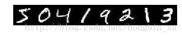
# 用一点小技巧来贴出前8张图片
imshow(solver.net.blobs['data'].data[:8, 0].transpose(1, 0, 2).reshape(28, 8*28), cmap='gray')
axis('off')
print 'train labels:', solver.net.blobs['label'].data[:8]
train labels: [ 5. 0. 4. 1. 9. 2. 1. 3.]
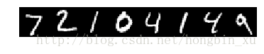
imshow(solver.test_nets[0].blobs['data'].data[:8, 0].transpose(1, 0, 2).reshape(28, 8*28), cmap='gray')
axis('off')
print 'test labels:', solver.test_nets[0].blobs['label'].data[:8]
test labels: [ 7. 2. 1. 0. 4. 1. 4. 9.]
4.分步运行solver
训练和测试网络都能正确导入数据和标签了。
- 使用SGD跑一次看看结果如何。
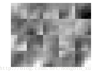
solver.step(1)# imshow(solver.net.params['conv1'][0].diff[:, 0].reshape(4,5,5,5).transpose(0,2,1,3).reshape(4*5, 5*5), cmap='gray')
# axis('off')
imshow(solver.net.params['conv1'][0].diff[:, 0].reshape(4, 5, 5, 5)
.transpose(0, 2, 1, 3).reshape(4*5, 5*5), cmap='gray'); axis('off')(-0.5, 24.5, 19.5, -0.5)
5.写一个训练的循环
一定发生了什么吧。我们花点时间跑跑这个网络,在它运行的同时也注意记录一些东西。注意,这里跟使用caffe编译好的二进制程序训练的过程是一样的。特别地:
- 终端依然会照常打印日志信息(logging)。
- snapshots(也就是保存中间过程产生的模型)会按照在solver prototxt文件中定义的间隔,比如这里是指每隔5000次迭代,取一次。
- 每过特定的间隔就会测试一次网络,这里是指500次迭代。
既然我们已经在Python代码中控制了循环操作,那么我们可以在运行程序的同时计算些别的东西了,如下所示。
我们也可以做些别的事,比如:
- 写一个停止循环的条件
- 在循环更新网络的同时改变解决方案的进程
%%time
niter = 200
test_interval = 25
# losses will also be stored in the log
train_loss = zeros(niter)
test_acc = zeros(int(np.ceil(niter / test_interval)))
output = zeros((niter, 8, 10))

# the main solver loop
for it in range(niter):
    solver.step(1)  # SGD by Caffe

    # store the train loss
    train_loss[it] = solver.net.blobs['loss'].data

    # store the output on the first test batch
    # (start the forward pass at conv1 to avoid loading new data)
    solver.test_nets[0].forward(start='conv1')
    output[it] = solver.test_nets[0].blobs['score'].data[:8]

    # run a full test every so often
    # (Caffe can also do this for us and write to a log, but we show here
    #  how to do it directly in Python, where more complicated things are easier.)
    if it % test_interval == 0:
        print 'Iteration', it, 'testing...'
        correct = 0
        for test_it in range(100):
            solver.test_nets[0].forward()
            correct += sum(solver.test_nets[0].blobs['score'].data.argmax(1)
                           == solver.test_nets[0].blobs['label'].data)
        test_acc[it // test_interval] = correct / 1e4
Iteration 0 testing...
Iteration 25 testing...
Iteration 50 testing...
Iteration 75 testing...
Iteration 100 testing...
Iteration 125 testing...
Iteration 150 testing...
Iteration 175 testing...
CPU times: user 1min 21s, sys: 68 ms, total: 1min 21s
Wall time: 1min 20s
- 接下来画出训练的loss和测试的准确率。
_, ax1 = subplots()
ax2 = ax1.twinx()
ax1.plot(arange(niter), train_loss)
ax2.plot(test_interval * arange(len(test_acc)), test_acc, 'r')
ax1.set_xlabel('iteration')
ax1.set_ylabel('train loss')
ax2.set_ylabel('test accuracy')
ax2.set_title('Test Accuracy: {:.2f}'.format(test_acc[-1]))
Text(0.5,1,u'Test Accuracy: 0.94')
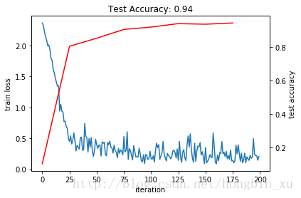
loss看起来下降的很快,也很快趋于收敛(当然要出去局部的随机性振荡),同时准确率也相应地提高了。万岁!
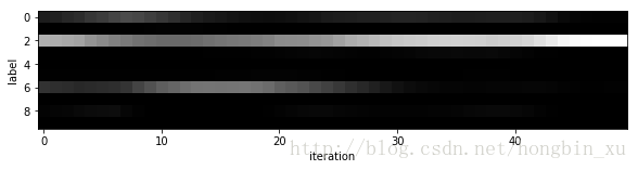
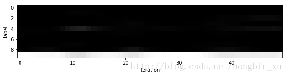
- 既然我们在第一个测试的batch中保存了结果,我们也当然可以看一下预测结果的变化。我们令x轴为时间,y轴对应每个可能的标签,亮度代表置信度。
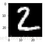
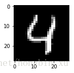
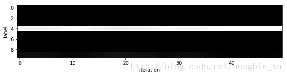
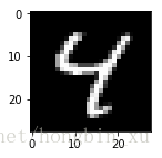
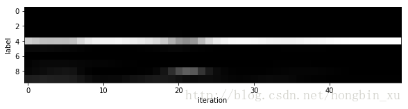
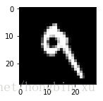
for i in range(8):
figure(figsize=(2,2))
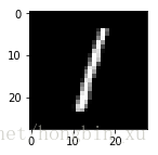
imshow(solver.test_nets[0].blobs['data'].data[i, 0], cmap='gray')
figure(figsize=(10,2))
imshow(output[150:200,i].T, interpolation='nearest', cmap='gray')
xlabel('iteration')
ylabel('label')
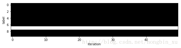

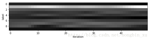
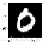


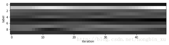


最初,我们几乎无法正确预测任何手写数字,最后慢慢的能够正确地分类他们了。如果你一直跟着教程走的话,你会看到最后的一个数字是最复杂的,一个倾斜的“9”,很容易被误认为是“4”
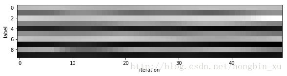
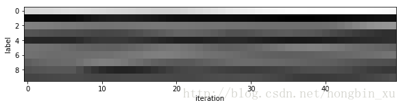
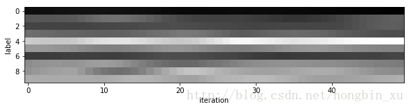
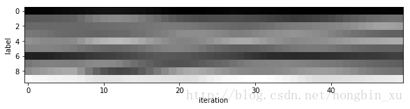
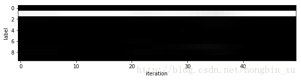
- 注意,这些都是神经网络最后的输出,而不是通过softmax计算后的向量。后者,正如下面所示,让我们更方便地看出网络的置信率。
for i in range(8):
    figure(figsize=(2,2))
    imshow(solver.test_nets[0].blobs['data'].data[i, 0], cmap='gray')
    figure(figsize=(10,2))
    imshow(exp(output[150:200,i].T) / exp(output[150:200,i].T).sum(0), interpolation='nearest', cmap='gray')
    xlabel('iteration')
    ylabel('label')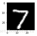


6.有关网络结构和优化的实验
现在我已经定义好了,分别用于训练和测试的LeNet网络,我们还有些别的事情要做:
- 定义新的结构,并与现在的对比效果
- 设置base_lr微调优化,或是再训练更长的时间
- 切换优化算法,比如使用AdaDelta或者Adam替换SGD
可以通过编辑下面的整合好的例子来试着自行探索。注释有“EDIT HERE”的地方是建议你修改的地方。
默认定义好了一个简单的线性分类器作为基线。
如果你更改的方案行不通,试着按照以下建议做做看:
1. 把非线性单元ReLU切换为ELU,或是一个基础的非线性单元,比如Sigmoid
2. 堆叠更多的全连接层和非线性层
3. 每次都试着10倍10倍地取学习率(比如0.1和0.001)
4. 切换优化算法为Adam(一般来说,这种自适应优化器对超参数不敏感,但也不保证一定如此…)
5. 多训练一段时间,把niter设置高一些(比如500或是1000)来看看差异
examples_path = '/home/xhb/caffe/caffe/examples/'
train_net_path = examples_path + 'mnist/custom_auto_train.prototxt'
test_net_path = examples_path + 'mnist/custom_auto_test.prototxt'
solver_config_path = examples_path + 'mnist/custom_auto_solver.prototxt'
### define net
def custom_net(lmdb, batch_size):
# define your own net!
n = caffe.NetSpec()
# keep this data layer for all networks
n.data, n.label = L.Data(batch_size=batch_size, backend=P.Data.LMDB, source=lmdb,
transform_param=dict(scale=1./255), ntop=2)
# EDIT HERE to try different networks
# this single layer defines a simple linear classifier
# (in particular this defines a multiway logistic regression)
n.score = L.InnerProduct(n.data, num_output=10, weight_filler=dict(type='xavier'))
# EDIT HERE this is the LeNet variant we have already tried
# n.conv1 = L.Convolution(n.data, kernel_size=5, num_output=20, weight_filler=dict(type='xavier'))
# n.pool1 = L.Pooling(n.conv1, kernel_size=2, stride=2, pool=P.Pooling.MAX)
# n.conv2 = L.Convolution(n.pool1, kernel_size=5, num_output=50, weight_filler=dict(type='xavier'))
# n.pool2 = L.Pooling(n.conv2, kernel_size=2, stride=2, pool=P.Pooling.MAX)
# n.fc1 = L.InnerProduct(n.pool2, num_output=500, weight_filler=dict(type='xavier'))
# EDIT HERE consider L.ELU or L.Sigmoid for the nonlinearity
# n.relu1 = L.ReLU(n.fc1, in_place=True)
# n.score = L.InnerProduct(n.fc1, num_output=10, weight_filler=dict(type='xavier'))
# keep this loss layer for all networks
n.loss = L.SoftmaxWithLoss(n.score, n.label)
return n.to_proto()
with open(train_net_path, 'w') as f:
f.write(str(custom_net('mnist/mnist_train_lmdb', 64)))
with open(test_net_path, 'w') as f:
f.write(str(custom_net('mnist/mnist_test_lmdb', 100)))
### define solver
from caffe.proto import caffe_pb2
s = caffe_pb2.SolverParameter()
# Set a seed for reproducible experiments:
# this controls for randomization in training.
s.random_seed = 0xCAFFE
# Specify locations of the train and (maybe) test networks.
s.train_net = train_net_path
s.test_net.append(test_net_path)
s.test_interval = 500 # Test after every 500 training iterations.
s.test_iter.append(100) # Test on 100 batches each time we test.
s.max_iter = 10000 # no. of times to update the net (training iterations)
# EDIT HERE to try different solvers
# solver types include "SGD", "Adam", and "Nesterov" among others.
s.type = "SGD"
# Set the initial learning rate for SGD.
s.base_lr = 0.01 # EDIT HERE to try different learning rates
# Set momentum to accelerate learning by
# taking weighted average of current and previous updates.
s.momentum = 0.9
# Set weight decay to regularize and prevent overfitting
s.weight_decay = 5e-4
# Set `lr_policy` to define how the learning rate changes during training.
# This is the same policy as our default LeNet.
s.lr_policy = 'inv'
s.gamma = 0.0001
s.power = 0.75
# EDIT HERE to try the fixed rate (and compare with adaptive solvers)
# `fixed` is the simplest policy that keeps the learning rate constant.
# s.lr_policy = 'fixed'
# Display the current training loss and accuracy every 1000 iterations.
s.display = 1000
# Snapshots are files used to store networks we've trained.
# We'll snapshot every 5K iterations -- twice during training.
s.snapshot = 5000
s.snapshot_prefix = 'mnist/custom_net'
# Train on the GPU
s.solver_mode = caffe_pb2.SolverParameter.GPU
# Write the solver to a temporary file and return its filename.
with open(solver_config_path, 'w') as f:
f.write(str(s))
### load the solver and create train and test nets
solver = None # ignore this workaround for lmdb data (can't instantiate two solvers on the same data)
solver = caffe.get_solver(solver_config_path)
### solve
niter = 250 # EDIT HERE increase to train for longer
test_interval = niter / 10
# losses will also be stored in the log
train_loss = zeros(niter)
test_acc = zeros(int(np.ceil(niter / test_interval)))
# the main solver loop
for it in range(niter):
solver.step(1) # SGD by Caffe
# store the train loss
train_loss[it] = solver.net.blobs['loss'].data
# run a full test every so often
# (Caffe can also do this for us and write to a log, but we show here
# how to do it directly in Python, where more complicated things are easier.)
if it % test_interval == 0:
print 'Iteration', it, 'testing...'
correct = 0
for test_it in range(100):
solver.test_nets[0].forward()
correct += sum(solver.test_nets[0].blobs['score'].data.argmax(1)
== solver.test_nets[0].blobs['label'].data)
test_acc[it // test_interval] = correct / 1e4
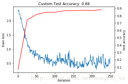
_, ax1 = subplots()
ax2 = ax1.twinx()
ax1.plot(arange(niter), train_loss)
ax2.plot(test_interval * arange(len(test_acc)), test_acc, 'r')
ax1.set_xlabel('iteration')
ax1.set_ylabel('train loss')
ax2.set_ylabel('test accuracy')
ax2.set_title('Custom Test Accuracy: {:.2f}'.format(test_acc[-1]))Iteration 0 testing...
Iteration 25 testing...
Iteration 50 testing...
Iteration 75 testing...
Iteration 100 testing...
Iteration 125 testing...
Iteration 150 testing...
Iteration 175 testing...
Iteration 200 testing...
Iteration 225 testing...
Text(0.5,1,u'Custom Test Accuracy: 0.88')