matplotlib（3.注释、文本、多边形、区域填充、极坐标）

更新一些matplotlib绘图周边内容

---

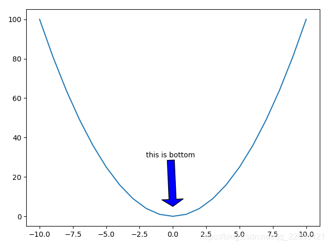
加箭头注释

import matplotlib.pyplot as plt
import numpy as np

x = np.arange(-10, 11, 1)

y = x**2

plt.plot(x, y)

# 设置显示文本：‘this is bottom’，设置指向位置xy，设置文本位置xytext，设置箭头参数（设置颜色：facecolor，设置箭头的头长：headlength，设置箭头的头宽：headwidth，设置箭头的体宽：width)
plt.annotate('this is bottom', xy=(0,5), xytext=(-2,30),
             arrowprops=dict(facecolor='b', headlength=10, headwidth=30,width=10))

plt.show()

加文本Text

例1：增加文字说明

import matplotlib.pyplot as plt
import numpy as np

x = np.arange(-10, 11, 1)

y = x**2

plt.plot(x, y)

# 显示位置x,y(2，40)，显示内容'function:y=x*x',字体family：serif，字号size：20，颜色color:'r',样式style:italic(斜体），字粗：black
plt.text(2, 40, 'function:y=x*x', family='serif', size=20, color='r', style='italic', weight='black')
plt.text(-7, 70, 'function:y=x*x', family='fantasy', size=30, color='g', style='oblique', weight='light', bbox=dict(facecolor='y', alpha=0.2))

plt.show()

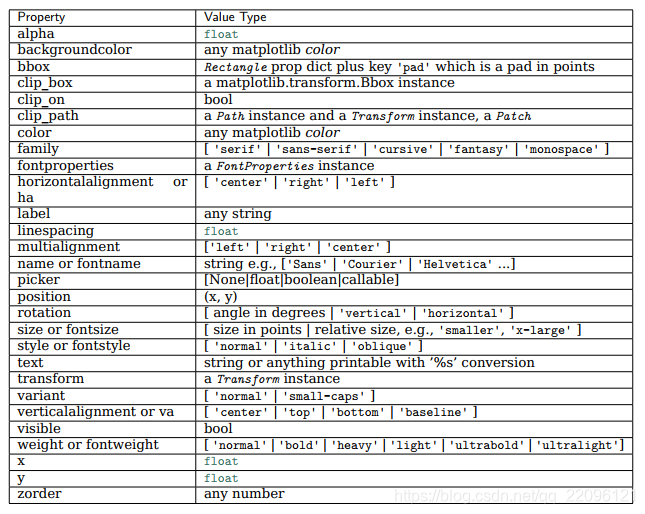
Text属性列表

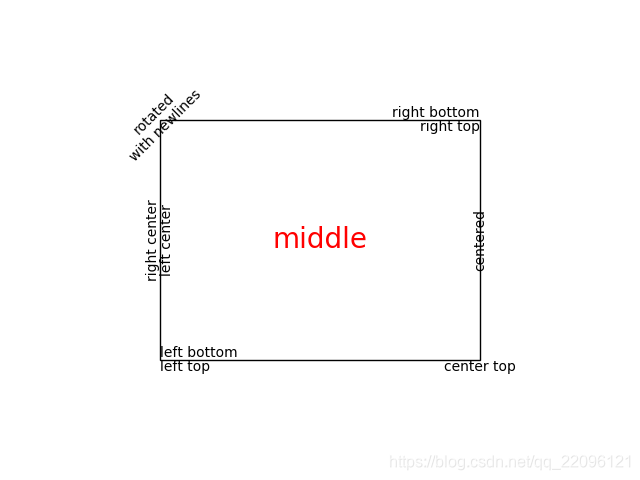
例2：developer guide给出例子

import matplotlib.pyplot as plt
import matplotlib.patches as patches

# build a rectangle in axes coords
left, width = .25, .5
bottom, height = .25, .5
right = left + width
top = bottom + height
fig = plt.figure()
ax = fig.add_axes([0, 0, 1, 1])
# axes coordinates are 0,0 is bottom left and 1,1 is upper right
p = patches.Rectangle(
    (left, bottom), width, height,
    fill=False, transform=ax.transAxes, clip_on=False
)
ax.add_patch(p)
ax.text(left, bottom, 'left top',
        horizontalalignment='left',
        verticalalignment='top',
        transform=ax.transAxes)
ax.text(left, bottom, 'left bottom',
        horizontalalignment='left',
        verticalalignment='bottom',
        transform=ax.transAxes)
ax.text(right, top, 'right bottom',
        horizontalalignment='right',
        verticalalignment='bottom',
        transform=ax.transAxes)
ax.text(right, top, 'right top',
        horizontalalignment='right',
        verticalalignment='top',
        transform=ax.transAxes)
ax.text(right, bottom, 'center top',
        horizontalalignment='center',
        verticalalignment='top',
        transform=ax.transAxes)
ax.text(left, 0.5 * (bottom + top), 'right center', horizontalalignment='right',
        verticalalignment='center',
        rotation='vertical',
        transform=ax.transAxes)
ax.text(left, 0.5 * (bottom + top), 'left center',
        horizontalalignment='left',
        verticalalignment='center',
        rotation='vertical',
        transform=ax.transAxes)
ax.text(0.5 * (left + right), 0.5 * (bottom + top), 'middle',
        horizontalalignment='center',
        verticalalignment='center',
        fontsize=20, color='red',
        transform=ax.transAxes)
ax.text(right, 0.5 * (bottom + top), 'centered',
        horizontalalignment='center',
        verticalalignment='center',
        rotation='vertical',
        transform=ax.transAxes)
ax.text(left, top, 'rotated\nwith newlines',
        horizontalalignment='center',
        verticalalignment='center',
        rotation=45,
        transform=ax.transAxes)
ax.set_axis_off()
plt.show()

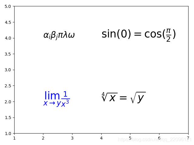
LaTeX公式

Writing mathematical expressions

和CSDN博客支持的LaTeX数学公式相同，这是一种单独的公式表示方式，可以自行搜索其语法。

例1：简单写四个公式demo

import matplotlib.pyplot as plt
import numpy as np

fig = plt.figure()

ax = fig.add_subplot(111)

ax.set_xlim([1, 7])

ax.set_ylim([1, 5])

ax.text(2, 4, r"$ \alpha_i \beta_j \pi \lambda \omega $",size=20)

ax.text(4,4, r"$ \sin(0)=\cos(\frac{\pi}{2}) $",size=25)

ax.text(2,2,r"$ \lim_{x \rightarrow y}\frac{1}{x^3}  $",size=25,color='b')

ax.text(4,2,r"$ \sqrt[4]{x}=\sqrt{y} $",size=25)
plt.show()

区域填充

fill, fill_between

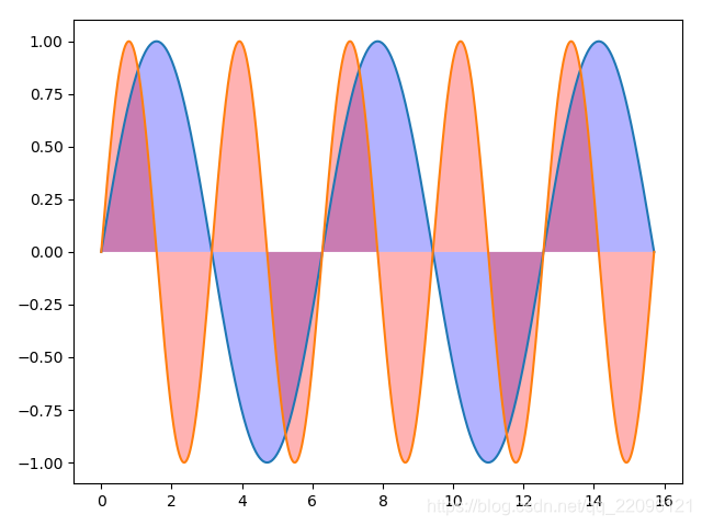
例1：fill函数方式

import matplotlib.pyplot as plt
import numpy as np

x = np.linspace(0,5*np.pi,1000)

y1 = np.sin(x)

y2 = np.sin(2*x)

plt.plot(x,y1)

plt.plot(x,y2)

plt.fill(x,y1,'b',alpha=0.3)

plt.fill(x,y2,'r',alpha=0.3)

plt.show()

可以看到：fill填充了函数与X轴之间的区域

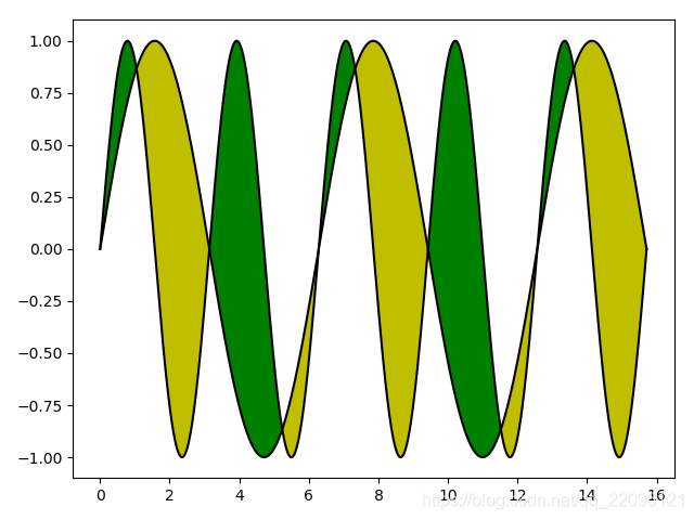
例2：fill_between

x = np.linspace(0,5*np.pi,1000)

y1 = np.sin(x)

y2 = np.sin(2*x)

fig = plt.figure()

ax = fig.gca()

ax.plot(x,y1,x,y2,color='black')

# 填充y1,y2之间，当y1>y2时，填充黄色，离散区域自动填充interpolate=True
ax.fill_between(x,y1,y2,where=y1>y2,facecolor='y',interpolate=True)

# 填充y1,y2之间，当y1<y2时，填充绿色，离散区域自动填充interpolate=True
ax.fill_between(x,y1,y2,where=y1<y2,facecolor='g',interpolate=True)
plt.show()

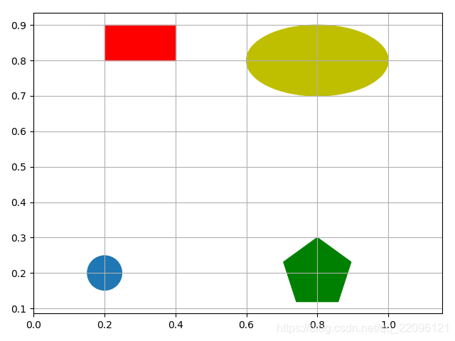
绘制多边图形

例1：绘制圆形，椭圆形，长方形，多边形

import matplotlib.pyplot as plt
import numpy as np
import matplotlib.patches as mpatches

fig, ax = plt.subplots()

# 指定图形位置
xy1 = np.array([0.2, 0.2])

# 圆半径0.05
circle = mpatches.Circle(xy1, 0.05)

ax.add_patch(circle)

# rectangle左下角位置
xy2 = np.array([0.2, 0.8])
# 长方形长0.2，宽0.1
rect = mpatches.Rectangle(xy2, 0.2, 0.1, color='r')
ax.add_patch(rect)

xy3 = np.array([0.8, 0.2])
# 多边形：5条边，图形中心到边的距离为0.1
polygon=mpatches.RegularPolygon(xy3,5,0.1,color='g')
ax.add_patch(polygon)

xy4=np.array([0.8,0.8])
# 椭圆长短直径0.4\0.2
ellipse=mpatches.Ellipse(xy4,0.4,0.2,color='y')
ax.add_patch(ellipse)

plt.axis('equal')
plt.grid()

plt.show()

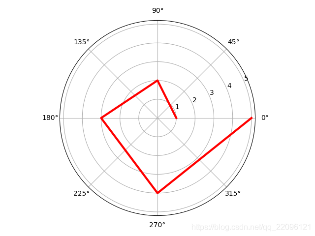
极坐标

确定角度和距离即可作图

例1：绘制距离1-5，角度0-2pi的图

r = np.arange(1, 6, 1)

theta = [0, np.pi / 2, np.pi, np.pi * 3 / 2, 2 * np.pi]

# 投影成极坐标=》projection='polar'
ax = plt.subplot(111, projection='polar')

ax.plot(theta, r, color='r', linewidth=3)

ax.grid(True)

plt.show()

后面开始更新实战例子