线性回归的常用求解方法之梯度下降法（二）：Python封装梯度下降线性回归

import numpy as np
import matplotlib.pyplot as plt
from sklearn.datasets import load_iris
from sklearn.model_selection import train_test_split
from sklearn.linear_model import SGDRegressor

iris = load_iris().data
#特征必须是二维的
feature = iris[:,2].reshape(-1,1)
#目标值可以是一维度
labels = iris[:,-1]

X_train,X_test,y_train,y_test = train_test_split(feature,labels,test_size=.3)

#fit_intercept不考虑误差   eta0=0.01 学习率
sgd = SGDRegressor(fit_intercept=False,eta0=0.01).fit(X_train,y_train)

sgd.score(X_train,y_train)

sgd.coef_,sgd.intercept_

#获取x轴的最大值和最小值
max_,min_ = feature.max()+1,feature.min()-1
#线型图需要向量
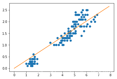
x = np.linspace(min_,max_,100)
y = sgd.coef_ * x
plt.plot(feature,labels,lw=0,marker='o')
plt.plot(x,y)

python实现梯度下降线性回归

• 1.误差问题:fit_intercept
• 2.迭代率:eat0
• 3.最大迭代次数，迭代次数越多(过拟合),越少(欠拟合)
• 4.增量式机器学习

class SGDLinearRegression(object):
    
    #构造函数
    def __init__(self,fit_intercept=True,eta0=0.01,max_iter=100):
        #全局属性
        self.fit_intercept = fit_intercept
        #迭代率
        self.eta0 =  eta0
        #最大迭代次数
        self.max_iter = max_iter
        
    #线性回归不是一个惰性学习
    def fit(self,X,y):
        #强制转换
        X = np.array(X)
        y = np.array(y)
        #获取特征和样本数量
        sample_sum,feature_nums = X.shape
        
        #将系数进行一个初始化的设定 ,一个有几个特征 那么 就有几个系数 矩阵(多行，1列)
        #初始化系数全部为0
        self.coef_ = np.zeros(shape=(feature_nums,1))
        #初始化误差为0  误差是一个常数项
        self.intercept_ = 0
        
        #添加一个数组，用于梯度下降的  残差 的记录
        self.save_loss_ = np.zeros(shape=self.max_iter)
        
        #梯度下降对比   真实目标值  和 预测目标值  残差
        for i in np.arange(self.max_iter):
            #预测的目标值
            h = np.add(np.dot(X,self.coef_),self.intercept_)
            
            #残差函数-->设置损失函数:  残差越大的话  系数和误差 向上增长的越快
            #传递了一个 特征数据   真实目标值  预测目标值  样本数量
            grad_w,grad_b,loss_ = self.loss(X,y,h,sample_sum)
            
            #粗调和精调
            self.coef_ -= self.eta0 * grad_w  
            
            if self.fit_intercept:
                self.intercept_ -= self.eta0 * grad_b
            else:
                self.intercept_ = 0
                
            #将系数转换成一位维的
        self.coef_ = self.coef_.ravel()
        return self
    #OOP思想，一个函数一件事
    def loss(self,X,y,h,sample_sum):
        #系数是二维的  特征也是二维  y有可能是一维    X 10 4   coef_  4 1  = (10,1)
        if y.ndim < 2:
            y = y.reshape(-1,1)
            
        #残差平方和
        #每一条数据相减  得到残差 
        #计算的是平fang误差   n条的数据误差相加的平方  除以  样本的数量  开根号
        loss = np.sqrt(np.divide(np.sum(np.square(np.subtract(y,h))),sample_sum))
        
        #调解系数增长
        grad_w = X.T.dot(h-y) / sample_sum
        
        #误差也需要增长
        grad_b = .5 * np.sum(h-y) / sample_sum
        
        return grad_w,grad_b,loss
    
    def predict(self,X):
        X = np.array(X)
        #获取预测目标值
        return X.dot(self.coef_) + self.intercept_

sgd_ = SGDLinearRegression(fit_intercept=False,eta0=0.01,max_iter=100).fit(X_train,y_train)

sgd_.coef_,sgd_.intercept_

#获取x轴的最大值和最小值
max_,min_ = feature.max()+1,feature.min()-1
#线型图需要向量
x = np.linspace(min_,max_,100)
y = sgd_.coef_* x
plt.plot(feature,labels,lw=0,marker='o')
plt.plot(x,y)