番外.李宏毅学习笔记.ST4.Sequence Labeling

公式输入请参考： 在线Latex公式
课程PPT

Sequence Labeling

Definition

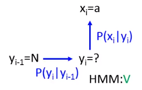
来看看定义（这里的定义其实并不严格，先暂时假定输入和输出的Sequence的长度都是相等的，为 $L$，实际上有很多种情况，其实在前面的课程有讲过）：

RNN can handle this task, but there are other methods based on structured learning(two steps, three problems).
典型应用：
•Name entity recognition
• Identifying names of people, places, organizations, etc.
from a sentence
• Harry Potter is a student of Hogwarts and lived on Privet Drive.
识别结果：
people: Harry Potter
organizations: Hogwarts
places: Privet Drive
not a name entity: 其他部分
但是对于中文的抽取很麻烦，例如下面两句要抽取人名：
楊公再興之神（出自金庸《笑傲江湖》）
馮氏埋香之塚（出自金庸《射雕英雄传》）
下面来看例子

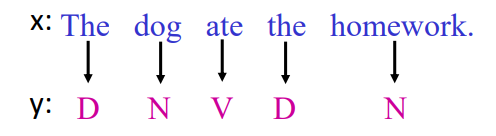
Example Task: POS tagging

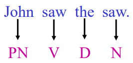
Annotate each word in a sentence with a part-of-speech.输入一个句子，输出每个词的类型，例如名词，动词什么的。
Useful for subsequent syntactic parsing and word sense disambiguation, etc.

下面是一个小例子，看到都是saw，有不一样的词性。

这个看起来很简单的东西，明显是不可以直接把词和词性保存下来，然后直接做简单的查询就行了。
“saw” is more likely to be a verb V rather than a noun N，为什么会知道第二个saw是名词呢？因为它在the后面
the second “saw” is a noun N because a noun N is more likely to follow a determiner.
也就是说词性和词序有很大关系。下面就将考虑词序的structed learning的技术依次介绍。

Hidden Markov Model (HMM)

先来看看人是如何构造一个句子：
Step 1
• Generate a POS sequence
• Based on the grammar
Step 2
• Generate a sentence based on the POS sequence
• Based on a dictionary
这实际上和HMM假设是一样的。

HMM – Step 1

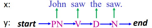
根据脑中的语法建立一个POS的sequence：

实际上这就是一个马尔科夫链，例如：
要说一句话，放在句首的0.5的几率是冠词，0.4的几率是专有名词，0.1的几率是动词
这里随机sample一下，假设第一个词是专有名词PN，PN后面80%几率是动词V，10%几率是冠词，10%几率直接结束。然后再随机sample一下。一直往下，直到end。
注意：每一个词后面接什么词合起来的几率应该是1，不是1就是ppt有问题。
当我们要计算"PN V D N"这样的一个序列的概率，就是上图中的式子。

HMM – Step 2

根据我们脑袋中的词典，把相应的词根据词性放到相应位置。

名词罐子里面有五个词，sample出John的几率是0.2，同理：得到saw的几率是0.17，the的几率是0.63，最后saw的几率是0.17，根据词性这句话出现的几率为：
$P(“John\space saw\space the\space saw“ | “PN\space V\space D\space N”) =0.2*0.17*0.63*0.17$

HMM的数学表达

HMM实际上就是在描述下面这件事情

数学表达为：
$P(x,y)=P(y)P(x|y)$
来看看右边分别怎么算的：
$P(y)=P(start)\times P(PN|start)\times P(V|PN)\times P(D|V)\times P(N|D)$
$P(x|y)=P(John|PN)\times P(saw|V)\times P(the|D)\times P(saw|N)$
用更加一般化的数学表达HMM：
输入： $x=x_1,x_2,...,x_L$
输出： $y=y_1,y_2,...,y_L$
step 1: （称为：Transition probability）
$P(y)=P(y_1)\times \prod_{l=1}^{L-1}P(y_{l+1}|y_l)\times P(end|y_L)\tag1$
step 2:（称为：Emission probability）
$P(x|y)=\prod_{l=1}^LP(x_l|y_l)\tag2$
写到一起：
$P(x,y)=P(y_1)\times \prod_{l=1}^{L-1}P(y_{l+1}|y_l)\times P(end|y_L)\prod_{l=1}^LP(x_l|y_l)\tag3$
怎么算这两个几率呢？

HMM– Estimating the probabilities

•Obtaining from training data
找一堆句子，并找砖家把每个词的词性标注出来。每一个句子就是一笔training data

那么算公式1中的 $P(y_{l+1}|y_l)$这个就是数数：
$P(y_{l+1}=s'|y_l=s)=\cfrac{count(s\to s')}{count(s)}$
$s$和 $s'$是tag（词性标签）
公式2中的 $P(x_l|y_l)$
$P(x_l=t|y_l=s)=\cfrac{count(s\to t)}{count(s)}$
$s$是tag（词性标签）， $t$是词。
讲到这里，老师解释了一下HMM在处理语音序列的时候表达式不是这样的，处理语音序列的时候，HMM里面的都是一个个搞屎分布形成的GMM，不是像这里用统计的方法算出来的，GMM要用EM来解，这里不用。为什么？老师也没说，自己想。。。
回到之前的POS tagging这个问题

现在 $y$是不知道的，也就是为什么叫Hidden的原因，现在我们知道怎么算 $P(x,y)$和 $x$，要求 $y$
用概率来说就是，在给定 $x$的条件下出现的几率的 $y$就是我们要求的 $y$
$y=arg\underset{y\in Y}{max}P(y|x)$
上式可以写成：
$y=arg\underset{y\in Y}{max}\cfrac{P(x,y)}{P(x)}$
由于分母 $P(x)$是固定的，所以上式等价于：
$y=arg\underset{y\in Y}{max}P(x,y)$
这个最有可能的 $y$就是穷举所有的 $y$，然后带入公式 $P(x,y)$里面，然后找到最大的那个~！，我们把它记为 $\tilde y$
下面来分析一下这个做法：

HMM – Viterbi Algorithm

$\tilde y=arg\underset{y\in Y}{max}P(x,y)$
• Enumerate all possible $y$会发生什么？
假设我们有 $S$个词性标签，sequence $y$长度为 $L$，那么 $y$的可能性就是：
$S^L$
这个玩意超大，不好算，于是有Viterbi Algorithm来解决这个问题，其算法时间复杂度为： $O(L(S)^2 )$

---

Viterbi-Algorithm算法
维特比算法是一个特殊但应用最广的动态规划算法。利用动态规划，可以解决任何一个图中的最短路径问题。而维特比算法是针对一个特殊的图-篱笆网了（Lattice）的有向图最短路径问题而提出来的。它之所以重要，是因为凡是使用隐马尔科夫模型描述的问题都可以用它解码，包括当前的数字通信、语音识别、机器翻译、拼音转汉字、分词等。
————————————————
版权声明：本文为CSDN博主「皮乾东」的原创文章，遵循 CC 4.0 BY-SA 版权协议，转载请附上原文出处链接及本声明。
原文链接：https://blog.csdn.net/meiqi0538/article/details/80960128

---

HMM - Summary

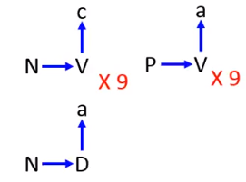
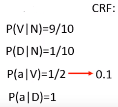
HMM的过程：

HMM的缺点：
假如输入 $x$对应的正确标签为 $\widehat y$，根据inference，我们希望 $\widehat y$的概率大于其他所有标签的概率：
$P(x,\widehat y)>P(x,y)$
但是这个式子不一定成立，因为 $P(x,y)$不一定很小，我们来看个例子：
Transition probability:
P(V|N)=9/10 P(D|N)=1/10 …
Emission probability:
P(a|V)=1/2 P(a|D)=1…
用图表示：

如下图所示，如果 $y_{l-1}=N$，在 $l$时刻观察到的 $x_l$是 $a$，那么 $y_l$最有可能是谁呢？

根据 $y_l=P(y_l|y_{l-1})\times P(x_l|y_l)$
如果放V， $y_l=0.9*0.5=0.45$
如果放D， $y_l=0.1*1=0.1$
按这个算法放V比较合适~！
现在我们来看看我们的training data是什么样子：

在training data中明显的出现的序列是： $N\to D\to a$，从来没有出现过： $N\to V\to a$，按HMM算法算出来来的序列却是： $N\to V\to a$，也就是说HMM算法只会按照概率的高低来进行估计，并不管这个序列是否出现过（HMM自己脑补了未出现过的东西）。这个脑补的过程也不能说就是个坏事
The $(x,y)$ never seen in the training data can have large probability $P(x,y)$.
•Benefit:
•When there is only little training data
由于训练数据很少，也就是意味在真实的数据中是有可能出现训练数据中没有出现过的序列的，因此HMM在训练数据很少的时候性能反而比较好。也就是说训练数据多的时候HMM的表现并没有比较好。
出现这个现象的根本原因是HMM把Transition probability和Emission probability是分开作为独立的概率来看待的，因此解决这个现象就是用更加复杂的模型，把这两个东西都考虑起来。
下面要讲的CRF就是用同样的模型，解决这个问题。

Conditional Random Field (CRF)

CRF也是要描述 $P(x,y)$，但是它描述的方式是：
$P(x,y)\propto\exp(w\cdot \phi(x,y))$
$\propto$是正比于的意思， $\phi(x,y)$是feature vector，
$w$ is a weight vector to be learned from training data，
$\exp(w\cdot \phi(x,y))$ 是一个正数，可以大于1.
下面是全概率公式出来：
$P(y|x)=\cfrac{P(x,y)}{\sum_{y'}P(x|y')}\tag4$
由于 $P(x,y)$和 $\exp(w\cdot \phi(x,y))$成正比，所以：
$P(x,y)=\cfrac{\exp(w\cdot \phi(x,y))}{R}\tag5$
把公式5带入4后，4中的分母互相消掉：
$P(y|x)=\cfrac{\exp(w\cdot \phi(x,y))}{\sum_{y'\in Y}\exp(w\cdot \phi(x,y'))}$
分母中是对所有的y进行求和，因此和x是相互独立的，可以把上式写成：
$P(y|x)=\cfrac{\exp(w\cdot \phi(x,y))}{Z(x)}$

P(x,y) for CRF

为什么说CRF和HMM是一样的呢？是有人证明了的，CRF只不过是training上不一样，我们来看，在HMM里面是这样计算 $P(x,y)$的
$P(x,y)=P(y_1)\times \prod_{l=1}^{L-1}P(y_{l+1}|y_l)\times P(end|y_L)\prod_{l=1}^LP(x_l|y_l)\tag3$
按乘法变加法的套路，对公式（3）的两边取对数
$logP(x,y)=logP(y_1)+\sum_{l=1}^{L-1}logP(y_{l+1}|y_l)+log P(end|y_L)+\sum_{l=1}^LlogP(x_l|y_l)\tag6$

---

最后一项：

解释一下：
$s$是词性标签
$t$是词表中所有的单词
如果 $s=10$， $t=1000$，那么 $\sum_{s,t}$一共有 $10×1000=10000$项
$logP(t|s)$：单词 $t$被标签为词性 $s$的概率取对数
$N_{s,t}(x,y)$：是单词 $t$被标签为词性 $s$这个事情，在 $(x,y)$中出现的次数

---

最后这一项 $N_{s,t}(x,y)$比较难理解，下面看一个具体的例子：

$N_{D,the}(x,y)=2$
$N_{N,dog}(x,y)=1$
$N_{V,ate}(x,y)=1$
$N_{N,homework}(x,y)=1$
$(for\space any\space other\space s\space and\space t),N_{s,t}(x,y)=0$
$\sum_{l=1}^LlogP(x_l|y_l)=logP(the,D)+logP(dog,N)+logP(ate,V)+logP(the,D)+logP(homework,N)\\ =logP(the,D)\times2+logP(dog,N)\times1+logP(ate,V)\times1+logP(homework,N)\times1\\ =\sum_{s,t}logP(t|s)\times N_{s,t}(x,y)$
公式（6）的前面三项分别为：
$logP(x,y)=logP(y_1)+\sum_{l=1}^{L-1}logP(y_{l+1}|y_l)+log P(end|y_L)+\sum_{l=1}^LlogP(x_l|y_l)\tag6$
$logP(y_1)=\sum_{s}logP(s|start)\times N_{start,s}(x,y)$
$\sum_{l=1}^{L-1}logP(y_{l+1}|y_l)=\sum_{s',s}logP(s'|s)\times N_{s',s}(x,y)$
$log P(end|y_L)=\sum_slogP(end|s)\times N_{s,end}(x,y)$
公式（6）可以写成一大堆两项的相乘：
$logP(x,y)=\sum_{s,t}logP(t|s)\times N_{s,t}(x,y)+\sum_{s}logP(s|start)\times N_{start,s}(x,y)+\sum_{s',s}logP(s'|s)\times N_{s',s}(x,y)+\sum_slogP(end|s)\times N_{s,end}(x,y)\\ =\begin{bmatrix} \vdots\\ logP(t|s)\\ \vdots\\ \vdots\\ logP(s|start)\\ \vdots\\ \vdots\\ logP(s'|s)\\ \vdots\\ \vdots\\ logP(end|s)\\\vdots\end{bmatrix}\cdot\begin{bmatrix} \vdots\\ N_{s,t}(x,y)\\ \vdots\\ \vdots\\ N_{start,s}(x,y)\\ \vdots\\ \vdots\\ N_{s',s}(x,y)\\ \vdots\\ \vdots\\ N_{s,end}(x,y)\\\vdots\end{bmatrix}\\ =w\cdot\phi(x,y)$

两边取指数e：
$P(x,y)=exp(w\cdot\phi(x,y))$
到这里就从HMM的形式推导到CRF的形式了，说明两个是一码事，但是注意，在CRF的定义中，上面的式子不是等号是正比于 $\propto$，下面看看为什么。
从上面矩阵化简的过程中，我们知道：
$\phi(x,y)=\begin{bmatrix} \vdots\\ N_{s,t}(x,y)\\ \vdots\\ \vdots\\ N_{start,s}(x,y)\\ \vdots\\ \vdots\\ N_{s',s}(x,y)\\ \vdots\\ \vdots\\ N_{s,end}(x,y)\\\vdots\end{bmatrix}$
$w=\begin{bmatrix} \vdots\\ logP(t|s)\\ \vdots\\ \vdots\\ logP(s|start)\\ \vdots\\ \vdots\\ logP(s'|s)\\ \vdots\\ \vdots\\ logP(end|s)\\\vdots\end{bmatrix}\tag7$
后面这个等式(7)中，每一个权重和几率是有对应关系的，把右边的log项取指数就把P前面的log变没有：

这里有点没明白，先记下来：
w在训练的过程中，我们并没有对其做任何限制，所以它可为正和负，如果为负，取指数后小于1，解释为几率没问题，但是如果它是正数的时候，取指数后是可能大于1的，也就是说下式的等号不一定成立，就该成了正比于。
$P(x,y)=exp(w\cdot\phi(x,y))$

Feature Vector

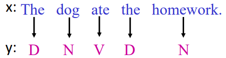
下面来看CRF的Feature Vector是什么样子，就是 $\phi(x,y)$这个东西。直接看例子：
假如输入输出 $(x,y)$如下图：

$\phi(x,y)$ has two parts
Part 1: relations between tags and words（是一个vector，它的dimension为： $s\times t$，其中 $s$是词性标签， $t$是词表中所有的单词，这个vector是很sparse的）

Part 2: relations between tags
$N_{s,s'}(x,y)$: Number of tags s and s’ consecutively in x,y
例如：下面 $N_{D,D}(x,y)=0$表示词性D出现在D后面在所有 $(x,y)$中出现的次数是0.
$N_{D,N}(x,y)=0$表示词性D出现在D后面在所有 $(x,y)$中出现的次数是2
这个玩意也是一个vector，他的维度为： $S\times S+2\times S$
意思是如果有 $S$个词性，每个词性之间都会有一个组合 $S\times S$，每个 $S$都和start有一个组合，和end有一个组合，就是 $2\times S$

最后要说的是，CRF牛叉的地方在于，这个特征向量可以不这样定义，可以自己来定义 $\phi(x,y)$的形式。

CRF – Training Criterion

下面来看CRF如何训练，假设我们有一组训练数据
$\{(x^1,\widehat y^1),(x^2,\widehat y^2),...,(x^N,\widehat y^N)\}$
Find the weight vector $w^*$ maximizing objective function $O(w)$:
$w^*=arg\underset{w}{max}O(w)$
$O(w)=\sum_{n=1}^NlogP(\widehat y^n|x^n)$
根据CRF的定义：
$logP(\widehat y^n|x^n)=log(\cfrac{P(x^n,\widehat y^n)}{\sum_{y'}P(x^n,y')})$
log中除法变减法：

下面看梯度如何求，由于上面是求最大值，所以是梯度上升求解Gradient Ascent：
Find a set of parameters $\theta$ maximizing objective function $O(\theta)$
$\theta\to\theta+\eta\triangledown O(\theta)$
下面看具体怎么弄，先写出目标函数：
$O(w)=\sum_{n=1}^NlogP(\widehat y^n|x^n)=\sum_{n=1}^NO^n(w)$
计算梯度
$\triangledown O^n(w)=\begin{bmatrix} \vdots\\ \cfrac{\partial O^n(w)}{\partial w_{s,t}}\\ \vdots\\ \cfrac{\partial O^n(w)}{\partial w_{s,s'}}\\ \vdots\\ \end{bmatrix}$
下面先看看 $\cfrac{\partial O^n(w)}{\partial w_{s,t}}$如何计算，另外一个 $\cfrac{\partial O^n(w)}{\partial w_{s,s'}}$是类似的，就不说了。（哭晕，具体过程在附录，没看懂，不贴过程了，上结果）
$\cfrac{\partial O^n(w)}{\partial w_{s,t}}=N_{s,t}(x^n,\widehat y^n)-\sum_{y'}P(y'|x^n)N_{s,t}(x^n,y')$
第一项：If word $t$ is labeled by tag $t$ in training examples $(x^n,\widehat y^n)$, then increase $w_{s,t}$
第二项：If word $t$ is labeled by tag $t$ in $(x^n,y')$ which not in training examples, then decrease $w_{s,t}$，这项也可以用Viterbi algorithm 来算
$\triangledown O(w)=\phi(x^n,\widehat y^n)-\sum_{y'}P(y'|x^n)\phi(x^n,y')$
Stochastic Gradient Ascent
$w\to w+\eta(\phi(x^n,\widehat y^n)-\sum_{y'}P(y'|x^n)\phi(x^n,y'))$

CRF – Inference

从HMM我们知道这个东西：
$y=arg\underset{y\in Y}{max}P(y|x)=arg\underset{y\in Y}{max}P(x,y)$
从CRF我们知道这个东西：
$P(x,y)\propto\exp(w\cdot \phi(x,y))$
所以有：
$y=arg\underset{y\in Y}{max}P(y|x)=arg\underset{y\in Y}{max}w\cdot\phi(x,y)$

CRF v.s. HMM

• CRF: increase $P(x,\widehat y)$, decrease $P(x,y')$
HMM does not decrease $P(x,y')$
之前说过，为了要获得正确的答案，我们需要使得正确的 $\widehat y$对应的几率要比其他所有的 $y$的几率要大：
$P(x,\widehat y)>P(x,y)$
由于CRF的特性，所以CRF的结果会比HMM的好。
例子：

HMM之前会脑补的情况：

如果是CRF，它会调整这些参数

最后结果是：

最后老师还讲了一下当初CRF提出来的论文，回顾了一下什么情况下CRF和HMM的性能怎么样。

CRF - Summary

把上面的过程整理下来，由于CRF也是属于机器学习的一种，因此我们也给它套上三板斧：

上面的 $w^*$用的是连乘，前面讲的时候是用的累加，其实是一样的，这里取log就变累加了，写法不一样，用累加性能好些，论文里面一般用连乘的写法。

Structured Perceptron/SVM

Structured Perceptron

也写出三板斧：
Problem 1: Evaluation
$F(x,y)=w\cdot\phi(x,y)$
这里的 $\phi(x,y)$可以自定义，如果不知道咋定义，可以直接和CRF定义一样的即可
Problem 2:Inference
$\tilde y=arg\underset{y\in Y}{max}w\cdot\phi(x,y)$
这个可以Viterbi算法来解
Problem 3: Training
$\forall n,\forall y\in Y,y\neq\widehat y^n:\\ w\cdot\phi(x^n,\widehat y^n)>w\cdot\phi(x^n,y)\\ \tilde y^n=arg\underset{y}{max}w\cdot\phi(x^n,y)$
$w\to w+\phi(x^n,\widehat y^n)-\phi(x^n,\tilde y^n)$
比较一下Structured Perceptron和CRF
Structured Perceptron:
$\tilde y^n=arg\underset{y}{max}w\cdot\phi(x^n,y)$
$w\to w+\phi(x^n,\widehat y^n)-\phi(x^n,\tilde y^n)$
CRF:
$w\to w+\eta(\phi(x^n,\widehat y^n)-\sum_{y'}P(y'|x^n)\phi(x^n,y'))$
如果不看CRF的学习率 $\eta$，发现两个参数更新的方式很像，其中 $\phi(x^n,\widehat y^n)$这项是一样的，后面那个不一样，直接的可以理解为：Structured Perceptron直接减掉错误几率的那个 $\tilde y$，CRF减掉所有错误的y的加权平均和，因此我们把 $\phi(x^n,\tilde y^n)$称为硬间隔， $\sum_{y'}P(y'|x^n)\phi(x^n,y')$软间隔。

Structured SVM

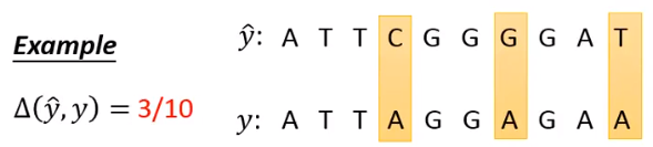
它的三板斧前面两板和Structured Perceptron的一样：
Problem 1: Evaluation
$F(x,y)=w\cdot\phi(x,y)$
这里的 $\phi(x,y)$可以自定义，如果不知道咋定义，可以直接和CRF定义一样的即可
Problem 2:Inference
$\tilde y=arg\underset{y\in Y}{max}w\cdot\phi(x,y)$
这个可以Viterbi算法来解
Problem 3: Training
Consider margin and error:
Way 1. Gradient Descent
Way 2. Quadratic Programming (Cutting Plane Algorithm)
Structured SVM还要考虑error：
Error function: $\Delta (\widehat y^n,y)$
$\Delta (\widehat y^n,y)$:Difference between $y$ and $y^n$
Structured SVM的cost函数就是 $\Delta (\widehat y^n,y)$的upper bound，也就是说cost函数实际上是最小化error的upper bound。
理论上， $\Delta (\widehat y^n,y)$可以我们自己随意定义，只要能衡量 $y$ and $y^n$之间的差异就可以。
但是我们要考虑解决Problem 2.1
$\bar y^n=arg\underset{y}{max}[\Delta (\widehat y^n,y)+w\cdot\phi(x^n,y)]$
下面是一个很好算的错误率 $\Delta (\widehat y^n,y)$

在这个情况下， problem 2.1 can be solved by Viterbi Algorithm

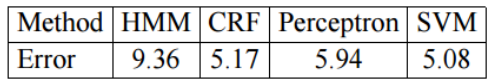
Performance of Different Approaches

POS Tagging
Ref: Nguyen, Nam, and Yunsong Guo. “Comparisons of sequence labeling algorithms and extensions.” ICML, 2007.

Name Entity Recognition
Ref: Tsochantaridis, Ioannis, et al. “Large margin methods for structured and interdependent output variables.” Journal of Machine Learning Research. 2005.

总结