模式识别:Python实现BP神经网络
前言:BP神经网络是理解神经网络原理的基础,代码实现有助于我们快速入门,深入理解。在此把本人在校期间模式识别的BP神经网络的作业题发出来和大家一起讨论,也望各位大佬指出不足之处,共同学习。
1.作业要求
-
请编写两个通用的三层前向神经网络反向传播算法程序,一个采用批量方式更新权重, 另一个采用单样本方式更新权重。其中,隐含层结点的激励函数采用双曲正切函数,输出 层的激励函数采用 sigmoid 函数。目标函数采用平方误差准则函数。
-
将数据带入所设计的BP神经网络
2.Python代码实现
"""
三层反向传播神经网络

批处理更新权重
不同的梯度更新步长对训练的影响

默认参数
rate= 0.001 0.004 0.006
node = 6
step = 5000
"""

import numpy as np
from numpy import dot, exp, ones, zeros, random, zeros_like, ones_like, multiply
import math
import matplotlib.pyplot as plt

# 给定数据  共三类,每类取7个作为训练数据,3个作为测试数据
class1 = np.array([[1.58, 2.32, -5.8], [0.67, 1.58, -4.78], [1.04, 1.01, -3.63],
                   [-1.49, 2.18, -3.39], [-0.41, 1.21, -4.73], [1.39, 3.16, 2.87],
                   [1.20, 1.40, -1.89], [-0.92, 1.44, -3.22], [0.45, 1.33, -4.38],
                   [-0.76, 0.84, -1.96]], dtype=float).reshape(-1, 3)

label1 = np.zeros_like(class1)
label1[:, 0] = ones([len(label1)], dtype=float)
class1 = np.hstack((class1, label1))

ext = np.ones(len(class1))
ext = ext.reshape(10, -1)
class1 = np.hstack((ext, class1))

class2 = np.array([[0.21, 0.03, -2.21], [0.37, 0.28, -1.8], [0.18, 1.22, 0.16],
                   [-0.24, 0.93, -1.01], [-1.18, 0.39, -0.39], [0.74, 0.96, -1.16],
                   [-0.38, 1.94, -0.48], [0.02, 0.72, -0.17], [0.44, 1.31, -0.14],
                   [0.46, 1.49, 0.68]]).reshape(-1, 3)

label2 = zeros_like(class2)
label2[:, 1] = ones([len(label2)], dtype=float)
class2 = np.hstack((ext, class2, label2))

class3 = np.array([[-1.54, 1.17, 0.64], [5.41, 3.45, -1.33], [1.55, 0.99, 2.69],
                   [1.86, 3.19, 1.51], [1.68, 1.79, -0.87], [3.51, -0.22, -1.39],
                   [1.40, -0.44, -0.92], [0.44, 0.83, 1.97], [0.25, 0.68, -0.99],
                   [0.66, -0.45, 0.08]]).reshape(-1, 3)

label3 = zeros_like(class3)
label3[:, 2] = ones([len(label3)], dtype=float)
class3 = np.hstack((ext, class3, label3))

#all_class = np.vstack((class1, class2, class3))
train_data = np.vstack((class1[:7], class2[:7], class3[:7]))
test_data = np.vstack((class1[7:], class2[7:], class3[7:]))

# 激励函数及相应导数
def tan_h(x):
    return math.tanh(x)

def diff_tang_h(x):
    return 1.0 / (1 + pow(x, 2))

# sigmoid
def sigmoid(x):
    return 1.0 / (1 + exp(-x))

# sigmoid 求导
def diff_sigmoid(x):
    out = sigmoid(x)
    return out * (1 - out)

# 线性函数
def linear(x):
    return x

# 线性函数求导
def diff_linear(x):
    return ones_like(x)  # 对线性函数求导 结果全是1

# 定义神经网络
class NN:
    # 输入层、隐藏层、输出层的节点(数)
    def __init__(self, n_i, n_h, n_o):

        # 获取各层节点数量
        self.n_i = n_i  # 还需 增加一个偏差节点
        self.n_h = n_h
        self.n_o = n_o

        # 激活神经网络的所有节点(向量) 存储加权求和之后 对应 net
        self.data_i = ones(self.n_i)  # n+1 x 1
        self.data_net_h = ones(self.n_h)  # node_num x 1
        self.data_net_o = ones(self.n_o)  # c x 1

        # 对应书上 y z
        self.data_y = ones(self.n_h)  # .reshape(-1,1)  # node_num x 1
        self.data_z = ones(self.n_o)  # c x 1

        self.f0_net_k = ones(self.n_o)
        self.delta_k = ones(self.n_o)

        # 初始化权重矩阵
        self.wi = random.random((self.n_h, self.n_i))  # 输入到隐含层权重  nxd
        self.wo = random.random((self.n_h, self.n_o))  # 隐含层到输出 nxc

        # 待更新缓存
        self.delta_wi_temp = self.wi
        self.delta_wo_temp = self.wo

    def calculate_output(self, input):  # 传进来单个样本 dx1
        # input layer
        self.data_i = input

        # in - hidden
        self.data_net_h = dot(self.wi, self.data_i)  # nxd x dx1 -- nx1
        self.data_y = np.array(list(map(tan_h, self.data_net_h)))

        # self.data_y = self.data_y.reshape(-1, 1)  # 初始化技巧! 1xn

        # hidden - output
        self.data_net_o = dot(self.data_y, self.wo)  # 1xn nxc
        self.data_z = list(map(sigmoid, self.data_net_o))
        return self.data_z  # 输出

    def BP(self, target, updata_flag, rate_1, rate_2):
        # -1 Layer Delta 计算更新量
        # get误差
        error_t_k = target - self.data_z
        for i in range(self.n_o):  # 对net k求导  1xc
            self.f0_net_k[i] = diff_sigmoid(self.data_net_o[i])

        self.delta_k = np.multiply(self.f0_net_k, error_t_k)
        data_y_temp = self.data_y.reshape(-1, 1)
        delta_wo = dot(data_y_temp, self.delta_k.reshape(1, 3))

        # -2 Layer Delta
        epsilon = zeros(self.n_h).reshape(-1, 1)  # n_hx1

        for i in range(self.n_h):
            epsilon[i] = multiply(self.delta_k, self.wo[i:i + 1][0]).sum()  # epsilon=(delta_k x wo[]) .sum   n x 1
        # print(epsilon)
        delta_wi = rate_2 * dot(epsilon, self.data_i.reshape(1, -1))

        self.delta_wo_temp = self.delta_wo_temp + delta_wo
        self.delta_wi_temp = self.delta_wi_temp + delta_wi

        if updata_flag == 1:
            # Updata
            # -1
            self.wo = self.wo + rate_2 * delta_wo
            # -2
            self.wi = self.wi + rate_1 * delta_wi

        error = 0.5 * dot((target - self.data_z), (target - self.data_z).reshape(-1, 1))

        return error

    def train(self, patterns, input_data, rate_1, rate_2):  # 输入全部样本

        stop_flag = 0
        error_set = []
        acc_set = []
        step = 0
        sample_len = len(patterns)
        sample_num = 0
        rate_temp = 0

        # while stop_flag == 0:
        for m in range(5000):
            step += 1
            updata_flag = 1

            for p in patterns:  # 样本集
                sample_num += 1
                inputs = p[1:4].reshape(-1, 1)  # 前三个是数据
                targets = p[4:]  # 后三个是目标 -标签

                if sample_num == sample_len:
                    updata_flag = 1

                self.calculate_output(inputs)  # 更新网络前向输出
                error = self.BP(targets, updata_flag, rate_1, rate_2)

            rate = self.test(input_data)
            rate_temp = rate_temp + rate

            if step % 100 == 0:
                error_set.append(error)
                print("error", error,"acc:",rate)
            if step % 10 == 0:
                rate_temp = rate_temp / 10
                acc_set.append(rate_temp)
                rate_temp = 0

        return error_set, acc_set

    def test(self, input_data):
        #  测试!!
        ok = 1
        for p in input_data:  # 测试样本集
            inputs = p[1:4].reshape(-1, 1)  # 前三个是数据
            targets = p[4:]  # 后三个是目标

            output = self.calculate_output(inputs)  # 更新网络前向输出
            out_class = np.where(output == np.max(output))

            if targets[out_class] == 1:
                ok = ok + 1
        rate = ok / len(input_data)
        return rate

    def plot_plot(self, error_set0, error_set1, error_set2):
        set_len = len(error_set1)

        plt.plot(range(set_len), error_set0, range(set_len), error_set1, '-', range(set_len), error_set2, '--')
        plt.legend(['rate1 = 0.001','rate2 = 0.004', 'rate3 = 0.006'], loc='best')
        plt.title("ErrorCurve")
        plt.show()


def Run(test_data=test_data):
    pat = train_data
    test_data = test_data

    rate_1 = 0.001
    rate_2 = 0.004
    rate_3 = 0.006

    # 创建一个神经网络:输入层  隐藏层  输出层
    n0 = NN(3, 3, 3)
    error_set0, acc0 = n0.train(pat, test_data, rate_2, rate_2)

    n1 = NN(3, 6, 3)
    error_set1, acc1 = n1.train(pat, test_data, rate_2, rate_2)

    n2 = NN(3, 8, 3)
    error_set2, acc2 = n1.train(pat, test_data, rate_2, rate_2)

    n2.plot_plot(acc0, acc1, acc2)


if __name__ == '__main__':
    Run()

# Liu Yaohua 2019.11.21 in UCAS
3.结果分析
(1)通过给定不同的rate,得到误差曲线如下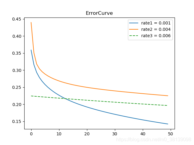
4.参考文献
《模式分类》 第二版
