Article Directory
1. How to deal with the data set?
from sklearn.dataset import load_iris # 加载鸢尾花数据集
When using scikit-learn, the data is usually represented by an uppercase X, and the label is represented by a lowercase y.
The train_test_split function of model_selection of scikit-learn can shuffle the data set and split it.
from sklearn.model_selection import train_test_split
X_train, X_test, y_train, y_test = train_test_split(
    iris_dataset['data'], iris_dataset['target'], random_state=0)
# 在对数据进行拆分之前,train_test_split 函数利用伪随机数生成器将数据集打乱
# random_state 参数指定了随机数生成器的种子。这样函数输出就是固定不变的
One of the best ways to check data is to visualize it. One visualization method is to draw a scatter plot. pandas has a function scatter_matrix() for drawing a scatter plot matrix. The diagonal of the matrix is a histogram of each feature.
# 利用DataFrame创建散点图矩阵,按y_train着色, 现在函数名为pd.plotting.scatter_matrix()
grr = pd.plotting.scatter_matrix(iris_dataframe, c=y_train, figsize=(15, 15), marker='o', hist_kwds={

    'bins': 20}, s=60, alpha=.8)
Scatter plot matrix:

2. How to call the algorithm?
All machine learning models in scikit-learn are implemented in their own classes, which are called Estimator classes. We need to instantiate this class as an object before we can use this model.
For example: the k-nearest neighbor classification algorithm is implemented in the KNeighborsClassifier class of the neighbors module.
from sklearn.neighbors import KNeighborsClassifier  # 加载实现KNN算法的类
knn = KNeighborsClassifier(n_neighbors=1)  # 创建一个实例对象,并初始化
knn.fit(X_train, y_train)
# 调用knn对象的fit方法,fit方法返回的是knn对象本身并做原处修改,得到了分类器的字符串表示。
y_pred = knn.predict(X_test) # 调用knn对象的predict方法,对验证集进行预测。
score = knn.score(X_test, y_test) # 调用knn对象的score方法,计算测试集的精度
np.mean(y_pred == y_test) # 另外一种计算测试集精度的方法
3. Supervised learning: classification and regression
There are two main types of supervised machine learning problems, called classification (classification) and regression (regression).
In the classification problem, the possible variety is called the class, and the variety with known data is called its label.
Classification tasks can sometimes be divided into
-
Two classification (binary classification, a special case of distinguishing between two categories)
Usually one of the categories is called the positive class, and the other is called the negative class.
-
Multi-classification (multiclass classification, distinguish between two or more categories)
The goal of the regression task is to predict a continuous value, the programming term is called floating-point number (floating-point number), and the mathematical term is called real number (real number).
A simple way to distinguish between classification tasks and regression tasks is to ask a question: Does the output have some continuity?
Constructing a model that is too complicated for the amount of information available is called overfitting.
Choosing a model that is too simple is called underfitting.
Overview of supervised learning algorithms:
| algorithm | to sum up |
|---|---|
| Nearest neighbor | Suitable for small data sets, it is a good benchmark model and easy to explain. |
| Linear model | Very reliable preferred algorithm, suitable for very large data sets, and also suitable for high-dimensional data. |
| Naive Bayes | Only applies to classification problems. It is faster than linear models and is suitable for very large data sets and high-dimensional data. The accuracy is usually lower than the linear model. |
| Decision tree | It is fast, does not require data scaling, can be visualized, and is easy to explain. |
| Random forest | Almost always better than a single decision tree, it is very robust and very powerful. No data scaling is required. Not suitable for high-dimensional sparse data. |
| Gradient Boosting Decision Tree | The accuracy is usually slightly higher than random forest. Compared with random forest, the training speed is slower, but the prediction speed is faster and requires less memory. It requires more parameter adjustments than random forests. |
| Support Vector Machines | It is powerful for medium-sized data sets with similar feature meanings. Data scaling is required and sensitive to parameters. |
| Neural Networks | Very complex models can be built, especially for large data sets. Sensitive to data scaling and parameter selection. |
Fourth, the main algorithm
4.1 Data set used
from sklearn.datasets import load_breast_cancer  # 威斯康星州乳腺癌数据集(用于分类数据集)
from sklearn.datasets import load_boston  # 波士顿房价数据集(用于回归数据集)
4.2 k nearest neighbors
The k-NN algorithm can be said to be the simplest machine learning algorithm.
from sklearn.neighbors import KNeighborsClassifier  # 用于分类的k近邻训练器
clf = KNeighborsClassifier(n_neighbors = 3)
from sklearn.neighbors import KNeighborsRegressor  # 用于回归的k近邻训练器
reg = KNeighborsRegressor(n_neighbors=3)
- k-nearest neighbor algorithm for classification
# 进行数据集的导入和拆分
from sklearn.datasets import load_breast_cancer
from sklearn.model_selection import train_test_split
cancer = load_breast_cancer()
X_train, X_test, y_train, y_test = train_test_split(cancer.data, cancer.target, stratify=cancer.target, random_state=66)
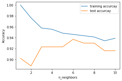
# 使用k近邻分类器训练邻居个数为1-10的模型,并计算准确率accuracy
from sklearn.neighbors import KNeighborsClassifier
training_accuracy = []
test_accuracy = []
neighbors_settings = range(1,11)
for n_neighbors in neighbors_settings:
    clf = KNeighborsClassifier(n_neighbors = n_neighbors)
    clf.fit(X_train, y_train)
    training_accuracy.append(clf.score(X_train, y_train))
    test_accuracy.append(clf.score(X_test, y_test))
plt.plot(neighbors_settings, training_accuracy, label="training accurcay")
plt.plot(neighbors_settings, test_accuracy, label="test accurcay")
plt.xlabel("n_neighbors")
plt.ylabel("Accuracy")
plt.legend()
Accuracy:
- k-nearest neighbor algorithm for regression
The prediction result using a single neighbor is the target value of the nearest neighbor. When multiple neighbors are used, the prediction result is the average of these neighbors. The specific code is consistent with the classification.
For regression problems, the score method of the evaluation model returns an R 2 score. The R 2 score is also called the coefficient of determination, which is a measure of the goodness of the regression model prediction, which lies between 0 and 1. R2 equal to 1 corresponds to a perfect prediction, and R2 equal to 0 corresponds to a constant model.
- to sum up
(1) Parameters: the number of neighbors and the measurement method of the distance between data points
(2) Advantages: easy to understand, good performance can be obtained without excessive adjustment, which is a good benchmark method.
(3) Disadvantages: The prediction speed is slow, and it is not suitable for training sets with many features, especially for sparse data sets.
4.3 Linear model
The linear model uses the linear function of the input features to make predictions.
from sklearn.linear_model import LinearRegression  # 线性回归的训练器
lr = LinearRegression()
from sklearn.linear_model import Ridge  # 岭回归的训练器
ridge = Ridge(alpha=1)
# alpha参数指定简单性和训练集性能二者对于模型的重要程度,alpha 的最佳设定值取决于具体数据集。
# 一般来说,alpha值越小模型越复杂,正则化越弱。
from sklearn.linear_model import Lasso  # Lasso回归的训练器
ridge = Ridge(alpha=0.01, max_iter=100000)
from sklearn.linear_model import LogisticRegression  # Logistic回归的分类器
logreg = LogisticRegression(C=1, penalty="l2")
# 参数C决定正则化强度的权衡参数,越大对应的正则化越弱;参数penalty决定选取正则化项类别
from sklearn.svm import LinearSVC   # 线性SVM的分类器,SVC代表支持向量分类器
The difference between linear model algorithms:
- A measure of how well a specific combination of coefficient and intercept fit the training data;
- Whether to use regularization, and which regularization method to use.
- Linear model for regression
For a linear model used for regression, the output ŷ is a linear function of the feature, which is a straight line, a plane, or a hyperplane (for higher-dimensional data sets). The prediction result of a single feature is a straight line, two features are a plane, or a hyperplane in a higher dimension (that is, more features).
If the number of features is greater than the number of training data points, any target y can be perfectly fitted (on the training set) with a linear function.
(I think it can be understood that the points in the training set are all on the regression curve!)
- Linear regression (also known as ordinary least squares (OLS))
Linear regression, or ordinary least squares method, is the simplest and most classic linear method for regression problems.
Linear regression looks for parameters w and b to minimize the mean square error between the predicted value of the training set and the true regression target value y .
The mean squared error is the sum of the squares of the difference between the predicted value and the true value divided by the number of samples.
# 线性回归过程
from sklearn.linear_model import LinearRegression
X, y = mglearn.datasets.make_wave(n_samples =60)
X_train, X_test, y_train, y_test = train_test_split(X,y,random_state=42)
lr = LinearRegression().fit(X_train, y_train)  # 创建线性回归分类器实例对象并训练
lr.coef_  # 该属性保存w,即权重或者系数
lr.intercept_  # 该属性保存b,即偏移或截距
lr.score(X_train, y_train)  # 计算训练集性能
lr.score(X_test, y_test)  # 计算测试集性能
The parameter w is stored in the coef_ attribute, which is a NumPy array, and each element corresponds to an input feature.
The parameter b is stored in the intercept_ attribute, which is a floating point number.
scikit-learn always saves the values derived from the training data in the attributes ending with an underscore. This is to distinguish it from the parameters set by the user.
- Ridge regression
In ridge regression, the choice of the coefficient ( w ) must not only get a good prediction result on the training data, but also fit additional constraints. We also hope that the coefficient is as small as possible. In other words, all elements of w should be close to zero.
The constraint of ridge regression is an example of regularization. Regularization refers to making explicit constraints on the model to avoid overfitting. This type of ridge regression is called L2 regularization.
from sklearn.linear_model import Ridge
ridge = Ridge(alpha=1)
Ridge regression and linear regression performance comparison:
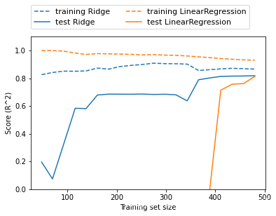
If there is enough training data, regularization becomes less important, and ridge regression and linear regression will have the same performance.
- lasso
lasso uses L1 regularization. The result of L1 regularization is that some coefficients are exactly 0 when using lasso. This shows that some features are completely ignored by the model. This can be seen as an automated feature selection.
from sklearn.linear_model import Lasso
ridge = Ridge(alpha=0.01, max_iter=100000)
The choice of ridge regression and lasso regression:
In practice, ridge regression is generally preferred in the two models. But if there are many features and you think only a few of them are important, then Lasso may be better. Similarly, if you want a model that is easy to explain, Lasso can give a model that is easier to understand because it only selects a part of the input features.
scikit-learn also provides the ElasticNet class, which combines the penalty items of Lasso and Ridge. In practice, this combination has the best effect, but at the cost of adjusting two parameters: one for L1 regularization and one for L2 regularization.
- Linear model for classification
- Linear model for binary classification
For linear models used for classification, the decision boundary is a linear function of the input. In other words, a (binary) linear classifier is a classifier that uses straight lines, planes, or hyperplanes to separate two categories.
The two most common linear classification algorithms are logistic regression (logistic regression) and linear support vector machine (linear support vector machine, linear SVM).
from sklearn.linear_model import LogisticRegression
from sklearn.svm import LinearSVC
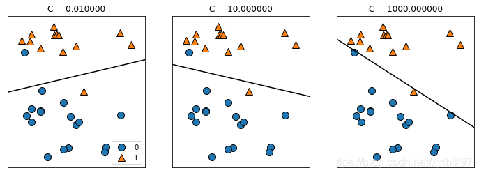
Both models use L2 regularization by default, and the trade-off parameter that determines the strength of regularization is called C. The larger the C value, the weaker the corresponding regularization. A small C value allows the algorithm to adapt to "most" data points as much as possible, while a larger C value emphasizes the importance of correct classification of each data point.
- Linear model for multiple classification
A common way to extend the two-classification algorithm to the multi-classification algorithm is the "one-vs.-rest" method. Run all second-class classifiers on the test points to make predictions. The classifier with the highest score in the corresponding category "wins" and returns this category label as the prediction result.
- to sum up
(1) The main parameter of the linear model is the regularization parameter, which is called alpha in the regression model, and C in LinearSVC and LogisticRegression. A larger alpha value or a smaller C value indicates that the model is relatively simple.
(2) The training speed of the linear model is very fast, and the prediction speed is also very fast. This model can be extended to very large data sets and is also effective for sparse data. The solver='sag' option, this option is faster than the default value when processing large data.
(3) Promotional version: SGDClassifier class and SGDRegressor class
4.4 Naive Bayes Classifier
Compared with the linear model, the naive Bayes classifier has faster training speed and slightly worse generalization ability.
Three naive Bayes classifiers are implemented in scikit-learn:
| name | Use range |
|---|---|
| GaussianNB | It can be applied to any continuous data, and the average and standard deviation of each feature in each category will be saved. |
| BernoulliNB | Assuming that the input data is two-category data, calculate the number of elements in each category with each feature that is not 0. |
| MultinomialNB | Assuming that the input data is count data, calculate the average of each feature in each category. |
All three classifiers have only one parameter alpha. The working principle of alpha is that the algorithm adds so many virtual data points with alpha to the data, and these points take positive values for all features. This can "smoothing" the statistics. The larger the alpha, the stronger the smoothing and the lower the model complexity.
- to sum up
The training and prediction speed of the naive Bayes model is very fast, and the training process is easy to understand.
The model has a good effect on high-dimensional sparse data, and its robustness to parameters is relatively good.
The Naive Bayes model is a good benchmark model and is often used for very large data sets.