Table of contents

1. Background description

The radius of curvature is a measure used to characterize the change of the degree of curvature at a certain point on the curve. It is an expression of sensitivity and can describe the equilibrium state of the system. From the perspective of data driving, it can be seen that the larger the range of data changes, the smaller the radius of curvature, and the worse the balance of the system; the smaller the range of data changes, the larger the radius of curvature, the better the balance of the system.
When the power grid is running in a stable state, the change range of the power grid state data is small and within a reasonable range. When the power grid is disturbed, the operating state of the power grid is prone to change, and the state data of the power grid response changes greatly. It can be seen that changes in system balance and stability will be accompanied by fluctuations in grid response data. From a data-driven point of view, the balance state and unbalance state of the power grid can be defined: in the balance state, the data is distributed in a reasonable range; in the unbalanced state, the quantitative data is distributed outside the reasonable range. Multi-dimensional data can use the main characteristic quantities and their changes in the state space to describe the balance of the system. The radius of curvature represents the physical state of the system in a mathematical sense. Considering the balance theory of the control system, this paper uses the radius of curvature as an evaluation index for system balance and imbalance. When the system data balance is poor, the corresponding data curvature radius is small; when When the balance of system data is good, the corresponding data has a large radius of curvature. In summary, when the radius of curvature of the system data is small, it can be judged as a weak link.

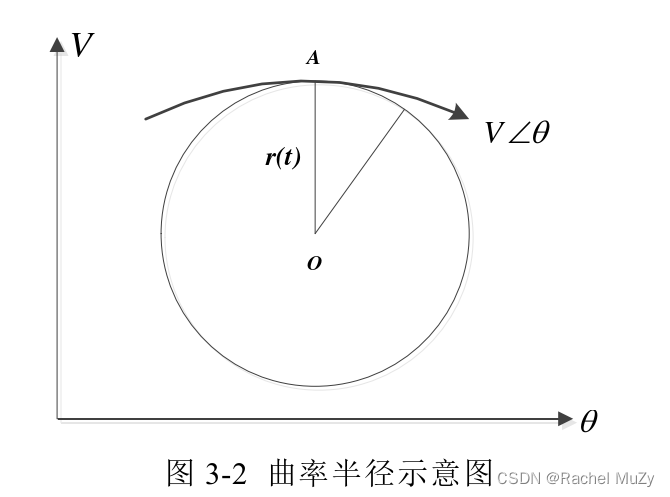
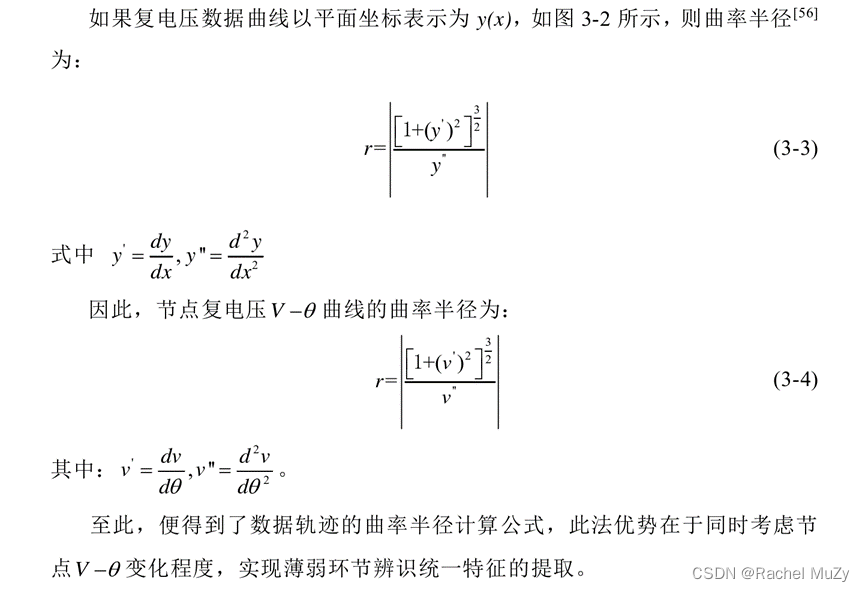
There is a strong coupling relationship between the components of the power grid, and a disturbance will cause the state of its links to change. The complex voltage data is used as the basic data of the unified analysis method for weak links in the power grid. The complex voltage data is the state data of the power grid operation process. The volatility and balance of data is an intuitive mapping of the operating state of the power grid. The research on complex voltage state data plays an important role in the analysis of power grid security and stability. In this paper, the curvature radius of node complex voltage data is used as a measure to measure its sensitivity change, that is, the curvature radius is used as the change characteristic of node complex voltage data.

2. Problem description

It is necessary to fit a curve function based on the existing discrete points, and then calculate the radius of curvature for each point.

3. Solutions

code:

import numpy as np
import matplotlib.pyplot as plt

#生成数据
x = np.linspace(0, np.pi, 10)
y = 5.0*np.cos(x)

#拟合曲线
fx = np.poly1d(np.polyfit(y,x,5))
dfx = fx.deriv()  # deriv()方法可得该格式函数的导函数
ddfx = dfx.deriv()

#求曲率半径
def calc_kappa(s):
    dx = dfx(s)
    ddx = ddfx(s)
    r = ((1 + (dx ** 2)) ** (3 / 2)) / ddx
    return r

snew = np.linspace(0, 10, 50)
k_buf = []
for i in snew:
    k = calc_kappa(i)
    k_buf.append(k)
k_buf = np.array(k_buf)
fig = plt.figure()
ax = fig.add_subplot(111)
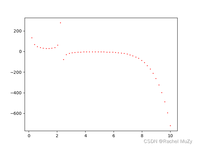
ax.scatter(snew[1:], k_buf[1:], s=1.0, color='red')
print(k_buf)
plt.show()

result:

[-6.53193563e+15  1.33313971e+02  6.81808541e+01  4.72685489e+01
  3.75737277e+01  3.26003863e+01  3.03470185e+01  3.02572039e+01
  3.27199881e+01  3.98667234e+01  6.16589764e+01  2.78196094e+02
 -7.62336205e+01 -2.92568474e+01 -1.67384408e+01 -1.11393142e+01
 -8.06852782e+00 -6.19380404e+00 -4.97862784e+00 -4.16929732e+00
 -3.63384573e+00 -3.30058795e+00 -3.13163381e+00 -3.11074516e+00
 -3.23787238e+00 -3.52716870e+00 -4.00701257e+00 -4.72131964e+00
 -5.73179385e+00 -7.12096897e+00 -8.99600601e+00 -1.14932740e+01
 -1.47837723e+01 -1.90794686e+01 -2.46406346e+01 -3.17842696e+01
 -4.08937100e+01 -5.24295296e+01 -6.69418450e+01 -8.50841470e+01
 -1.07628790e+02 -1.35484278e+02 -1.69714487e+02 -2.11559997e+02
 -2.62461671e+02 -3.24086684e+02 -3.98357149e+02 -4.87481563e+02
 -5.93989251e+02 -7.20768017e+02]

Notice:

The first one is not drawn here because the absolute value of the radius of curvature of the first point is extremely large: -6.53193563e+15. If drawn, it would look like this:

code:

import numpy as np
import matplotlib.pyplot as plt

#生成数据
x = np.linspace(0, np.pi, 10)
y = 5.0*np.cos(x)

#拟合曲线
fx = np.poly1d(np.polyfit(y,x,5))
dfx = fx.deriv()  # deriv()方法可得该格式函数的导函数
ddfx = dfx.deriv()

#求曲率半径
def calc_kappa(s):
    dx = dfx(s)
    ddx = ddfx(s)
    r = ((1 + (dx ** 2)) ** (3 / 2)) / ddx
    return r

snew = np.linspace(0, 10, 50)
k_buf = []
for i in snew:
    k = calc_kappa(i)
    k_buf.append(k)
k_buf = np.array(k_buf)
fig = plt.figure()
ax = fig.add_subplot(111)
ax.scatter(snew, k_buf, s=1.0, color='red')
print(k_buf)
plt.show()

result:

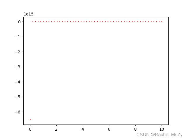
In this way, no other changes can be seen. So when processing, the first point is not drawn. As shown below:

[Machine Learning] python implements discrete point fitting curve and finds the radius of curvature

1. Background description

2. Problem description

3. Solutions

Guess you like