图像处理作业5——SIFT算法与全景图像生成

在这里插入图片描述

前前后后花了差不多两周的时间，终于完成了最后一个图像处理大作业，由于自己太菜，这个作业属实有点难顶哦，不过还好成功实现并按时提交，为自己干杯，哈哈！本篇博客记录自己的学习笔记及过程，以备以后回味和复习。

IDE：Jupyter notebook

题目：用手机或者相机拍摄不同角度图像（彼此之间有一定的重叠），用SIFT算子提取特征，通过特征匹配、图像旋转和图像融合等操作，将图像拼接在一起，形成大场景图像。

1. 实验思路

（1）尝试采用SIFT特征描述子提取特征；

（2）尝试特征匹配；

（3）找到变换矩阵，变换图像；

（4）拼接融合图像。

2. 实验原理

SIFT算法简介

SIFT (Scale-invariant feature transform)尺度不变特征转换即是一种计算机视觉的算法。它用来侦测与描述影像中的局部性特征，它在空间尺度中寻找极值点，并提取出其位置、尺度、旋转不变量，此算法由 David Lowe在1999年所发表，2004年完善总结。

扫描二维码关注公众号，回复： 11229916 查看本文章

SIFT算法的实质是在不同的尺度空间上查找关键点(特征点)，并计算出关键点的方向。SIFT所查找到的关键点是一些十分突出，不会因光照，仿射变换和噪音等因素而变化的点，如角点、边缘点、暗区的亮点及亮区的暗点等。

SIFT算法的特点有：

SIFT特征是图像的局部特征，其对旋转、尺度缩放、亮度变化保持不变性，对视角变化、仿射变换、噪声也保持一定程度的稳定性；
独特性（Distinctiveness）好，信息量丰富，适用于在海量特征数据库中进行快速、准确的匹配；
多量性，即使少数的几个物体也可以产生大量的SIFT特征向量；
高速性，经优化的SIFT匹配算法甚至可以达到实时的要求；
可扩展性，可以很方便的与其他形式的特征向量进行联合。

算法流程

在这里插入图片描述

SIFT算法实现物体识别主要有三大工序，1、提取关键点；2、对关键点附加详细的信息（局部特征）也就是所谓的描述器；3、通过两方特征点（附带上特征向量的关键点）的两两比较找出相互匹配的若干对特征点，也就建立了景物间的对应关系。

SIFT算法操作步骤

1. 关键点检测

1.1 哪些是SIFT中要查找的关键点（特征点）？

所为关键点，就是在不同尺度空间的图像下检测出的具有方向信息的局部极值点。可以得出关键点具有的三个特征：尺度、方向、大小。

1.2 什么是尺度空间（scale space）？

尺度空间理论最早是在1962年提出，其主要思想是通过对原始图像进行尺度变换，获得图像多尺度下的尺度空间表示序列，对这些序列进行尺度空间主轮廓的提取，并以该主轮廓作为一种特征向量，实现边缘、角点检测和不同分辨率上的特征提取等。

尺度空间中各尺度图像的模糊程度逐渐变大，能够模拟人在距离目标由近到远时目标在视网膜上的形成过程。尺度越大，图像越模糊。

高斯核是唯一可以产生多尺度空间的核，一个图像的尺度空间， $L(x,y,\sigma)$ ，定义为原始图像 $I(x,y)$ 与一个可变尺度的2维高斯函数 $G(x,y,\sigma)$ 卷积运算。高斯函数定义为：

$G(x_i,y_i,\sigma)=\frac{1}{2\pi\sigma^2}exp(-\frac{(x-x_i)^2=(y-y_i)^2}{2\sigma^2})$

$L(x,y,\sigma)=G(x,y,\sigma)*I(x,y)$

尺度是自然存在的，不是人为创造的！高斯卷积只是表现尺度空间的一种形式……

1.3 高斯模糊

高斯模糊通常用来减小图像噪声以及降低细节层次，这种模糊技术生成的图像的视觉效果是好像经过一个半透明的屏幕观察图像。

$G(r)=\frac{1}{2\pi\sigma^2}exp(-\frac{r^2}{2\sigma^2})$

$r$ 为模糊半径， $r=\sqrt{x^2+y^2}$

在实际应用中，在计算高斯函数的离散近似值时，在大概 $3\sigma$ 距离之外的像素都可以看作不起作用，这些像素的计算就可以忽略。

对一幅图像进行多次连续高斯模糊的效果与一次更大的高斯模糊可以产生同样的效果。例如，使用半径为6和8的两次高斯模糊变换得到的效果等同于一次半径为10的高斯模糊效果， $\sqrt{6^2+8^2}=10$ 。

1.4 高斯金字塔

高斯金字塔的构建过程可分为两步：（1）对图像做高斯平滑；（2）对图像做降采样。为了让尺度体现连续性，在简单下采样的基础上加上了高斯滤波。一幅图像可以产生几组（octave）图像，一组图像包括几层（interval）图像。

在这里插入图片描述

高斯金字塔共o组、s层，则有： $\sigma(s)=\sigma_02^\frac{s}{S}$ ，

$\sigma$ ——尺度空间坐标；s——sub-level层坐标； $\sigma_0$ ——初始尺度； $S$ ——每组层数（一般为3~5层）。

高斯金字塔的组内尺度与组间尺度：组内尺度是指同一组（octave）内的尺度关系， $\sigma_{s+1}=\sigma_s2^\frac{1}{S}$ ，组间尺度是指不同组直接的尺度关系，相邻组的尺度可化为： $\sigma_{o+1}(s)=\sigma_o2^\frac{s+S}{S}$ ， $\sigma_o2^\frac{s+S}{S}=2\sigma_o2^\frac{s}{S}$ 。由此可见，相邻两组的同一层尺度为2倍关系。

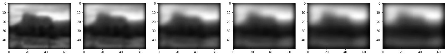
1.5 差分高斯金字塔

差分金字塔的是在高斯金字塔的基础上操作的，其建立过程是：在高斯金子塔中的每组中相邻两层相减（下一层减上一层）就生成高斯差分金字塔.高斯差分金字塔其操作如下图：

在这里插入图片描述

我们可以通过高斯差分金字塔图像看出图像上的像素值变化情况。（如果没有变化，也就没有特征。特征必须是变化尽可能多的点。）DOG图像描绘的是目标的轮廓。

在Lowe的论文中，将第0层的初始尺度定为1.6，图片的初始尺度定位0.5，则图像金字塔第0层的实际尺度为 $\sqrt{1.6*1.6-0.5*0.5}=1.52$ ，在检测极值点前对原始图像的高斯平滑以致图像丢失高频信息，所以Lowe建议在建立尺度空间前首先对原始图像长宽扩展一倍，以保留原始图像信息，增加特征点数量。当对图像长宽扩展一倍时，便构建了-1层，该层尺度为 $\sqrt{1.6*1.6-(2*0.5)*(2*0.5)}=1.25$

1.6 极值点检测

关键点是由DOG空间的局部极值点组成的，关键点的初步探查是通过同一组内各DOG相邻两层图像之间比较完成的。为了寻找DOG函数的极值点，每一个像素点要和它所有的相邻点比较，看其是否比它的图像域和尺度域的相邻点大或者小。如图下图所示，中间的检测点和它同尺度的8个相邻点和上下相邻尺度对应的9×2个点共26个点比较，以确保在尺度空间和二维图像空间都检测到极值点。

在这里插入图片描述

1.7 关键点精确定位

由于DOG值对噪声和边缘较敏感，因此，在上面DOG尺度空间中检测到局部极值点还要经过进一步的检验才能精确定位特征点。为了提高关键点的稳定性，需要对尺度空间DOG函数进行曲线拟合。利用DOG函数在尺度空间的Taylor展开式(插值函数)为：

任意一极值点在其 $X 0=(x 0, \quad y 0, \quad \sigma 0)$ 处泰勒展开并舍掉 2 阶以后的项结果如下： $f\left(\left[\begin{array}{l}x \\ y \\ \sigma\end{array}\right]\right) \approx f\left(\left[\begin{array}{l}x_{0} \\ y_{0} \\ \sigma_{0}\end{array}\right]\right)+\left[\begin{array}{lll}\frac{\partial f}{\partial x} & \frac{\partial f}{\partial y} & \frac{\partial f}{\partial \sigma}\end{array}\right]\left(\left[\begin{array}{l}x \\ y \\ \sigma\end{array}\right]-\left[\begin{array}{l}x_{0} \\ y_{0} \\ \sigma_{0}\end{array}\right]\right)$

$\left.\frac{1}{2}\left([\begin{array}{ccccccc}x & y & \sigma\end{array}\right]-\left[\begin{array}{ccc}x_{0} & y_{0} & \sigma_{0}\end{array}\right]\right)\left[\begin{array}{ccc}\frac{\partial^{2} f}{\partial x \partial x} & \frac{\partial^{2} f}{\partial x \partial y} & \frac{\partial^{2} f}{\partial x \partial \sigma} \\ \frac{\partial^{2} f}{\partial x \partial y} & \frac{\partial^{2} f}{\partial y \partial y} & \frac{\partial^{2} \pi}{\partial y \partial \sigma} \\ \frac{\partial^{2} f}{\partial x \partial \sigma} & \frac{\partial^{2} f}{\partial y \partial \sigma} & \frac{\partial^{2} f}{\partial \sigma \partial \sigma}\end{array}\right]\left(\left[\begin{array}{l} x \\ y \\ \sigma \end{array}\right]-\left[\begin{array}{l} x_{0} \\ y_{0} \\ \sigma_{0} \end{array}\right]\right)$

其中 f 的一阶偏导数，二阶偏导数，以及二阶混合偏导数由下面几个公式求（h=1）得：

$\frac{\partial f}{\partial x}=\frac{f(i, j+1)-f(i, j-1)}{2 h}, \quad \frac{\partial f}{\partial y}=\frac{f(i+1, j)-f(i-1, j)}{2 h}$

$\frac{\partial^{2} f}{\partial x^{2}}=\frac{f(i, j+1)+f(i, j-1)-2 f(i, j)}{h^{2}}, \quad \frac{\partial^{2} f}{\partial y^{2}}=\frac{f(i+1, j)+f(i-1, j)-2 j}{h^{2}}$

$\frac{\partial^{2} f}{\partial x \partial y}=\frac{f(i-1, j-1)+f(i+1, j+1)-f(i-1, j+1)-f(i+1, j-1)}{4 h^{2}}$

上面算式的矩阵表示如下：

$D(X)=D+\frac{\partial D^{T}}{\partial X} X+\frac{1}{2} X^{T} \frac{\partial^{2} D}{\partial X^{2}} X$ ，其中，X求导并让方程等于0，可得极值点的偏移量为 $\hat{X}=-\frac{\partial^{2} D^{-1}}{\partial X^{2}} \frac{\partial D}{\partial X}$ ，对应极值点，方程的值为 $D(\hat{X})=D+\frac{1}{2} \frac{\partial D^{T}}{\partial X} \hat{X}$

其中, $\hat{X}$ 代表相对插值中心的偏移量, 当它在任一维度上的偏移量大于0.5时 (即 $x$ 或 $y$ 或 $\sigma$ )，意味着插值中心已经偏移到它的邻近点上, 所以必须改变当前关键点的位置。同时在新的位置上反复插值直到收敛；也有可能超出所设定的迭代次数或者超出图像边界的范围, 此时这样的点应该删除, 在Lowe中进行了5次迭代。另外, 过小的点易受噪声的于扰而变得不稳定, 所以将小于某个经验值(Lowe论文中使用 $0.03$ ，Rob Hess等人实现时使用 $0.04/S$ )的极值点删除。同时, 在此过程中获取特征点的精确位置(原位置加上拟合的偏移量以及尺度( $\sigma$ )。

2. 关键点描述

2.1 关键点方向匹配

为了使描述符具有旋转不变性，需要利用图像的局部特征为给每一个关键点分配一个基准方向。使用图像梯度的方法求取局部结构的稳定方向。

（1）梯度计算

对于在DOG金字塔中检测出的关键点，采集其所在高斯金字塔图像 $3σ$ 领域窗口内像素的梯度和方向分布特征。梯度的模值和方向如下：

在这里插入图片描述

（2）梯度直方图

直方图以每10度方向为一个柱，共36个柱，柱所代表的的方向为像素点梯度方向，柱的长短代表了梯度幅值。
根据Lowe的建议，直方图1统计半径采用 $3*1.5*\sigma$ 。
在直方图统计时每相邻三个像素点采用高斯加权，模板采用 $[0.25,0.5,0.25]$ ，并连续加权两次。

在这里插入图片描述

（3）特征点主方向的确定

方向直方图的峰值则代表了该特征点处邻域梯度的方向，以直方图中最大值作为该关键点的主方向。为了增强匹配的鲁棒性，只保留峰值大于主方向峰值80％的方向作为该关键点的辅方向。因此，对于同一梯度值的多个峰值的关键点位置，在相同位置和尺度将会有多个关键点被创建但方向不同。仅有15％的关键点被赋予多个方向，但可以明显的提高关键点匹配的稳定性。实际编程实现中，就是把该关键点复制成多份关键点，并将方向值分别赋给这些复制后的关键点，并且，离散的梯度方向直方图要进行插值拟合处理，来求得更精确的方向角度值。

为了防止某个梯度方向角度因受到噪声的干扰而突变，我们还需要对梯度方向直方图进行平滑处理，平滑公式为：

$H(i)=\frac{h(i-2)+h(i+2)}{16}+\frac{4 \times(h(i-1)+h(i+1))}{16}+\frac{6 \times h(i)}{16}$

其中i∈[0,35], $h$ 和 $H$ 分别表示平滑前和平滑后的直方图。由于角度是循环的，即 $0^{\circ}=360^{\circ}$ ，如果出现 $h(j)$ ，j超出了(0,…,35)的范围，那么可以通过圆周循环的方法找到它所对应的、在 $0^{\circ}=360^{\circ}$ 之间的值，如h(-1) = h(35)。

（4）梯度直方图抛物线插值

在这里插入图片描述

假设我们在第i个小柱子要找一个精确的方向，那么由上面分析知道：设插值抛物线方程为 $h(t)=at^2-bt+c$ ,其中 $a、b、c$ 为执物线的系数， $t$ 自变量, $t\in[-1,1]$ ,此抛物线求导并令它等于0。
即 $h(t)'=0$ 得 $t_max=-b/(2a)$ 。现在把这三个插值点代入方程可得：

$\left.\begin{array}{l}\mathrm{h}(-1)=\mathrm{a}-\mathrm{b}+\mathrm{c} \\ \mathrm{h}(0)=\mathrm{c} \\ \mathrm{h}(1)=\mathrm{a}+\mathrm{b}+\mathrm{c}\end{array}\right\}$ ——> $\left\{\begin{array}{l}-\mathrm{a}=[\mathrm{h}(1)+\mathrm{h}(-1)] / 2-\mathrm{h}(0) \\ \mathrm{b}=[\mathrm{h}(1)-\mathrm{h}(-1)] / 2 \\ \mathrm{c}=\mathrm{h}(0)\end{array}\right.$

由上式知： $\mathrm{t}_{\mathrm{max}}=-\mathrm{b} /(2 \mathrm{a})=\frac{h(-1)-h(1)}{2[h(-1)+h(1)-2 h(0)]}$ （局部坐标系中的取值）

$\mathbf{i}^{\prime}=\mathbf{i}+\frac{h(i-1)-h(i+1)}{2[h(i-1)+h(i+1)-2 h(i)]}$ （小柱子在直方图中的索引号）。

图像的关键点已检测完毕，每个关键点有三个信息：位置、尺度、方向；同时也就使关键点具备平移、缩放、旋转不变性。

2.2 生成描述符

（1）确定计算描述子所需的区域

描述子梯度方向直方图由关键点所在尺度的模糊图像计算产生。图像区域的半径通过下式计算：

radius $=\frac{3 \sigma_{\text {oct}} \times \sqrt{2} \times(d+1)+1}{2}$ ， $\sigma_{oct}$ 是关键点所在组（octave）的组内尺度， $d=4$ 。

在这里插入图片描述

（2）将坐标移至关键点主方向

在这里插入图片描述

旋转角度后新坐标： $\left(\begin{array}{c}\hat{x} \\ \hat{y}\end{array}\right)=\left(\begin{array}{cc}\cos \theta & -\sin \theta \\ \sin \theta & \cos \theta\end{array}\right) \times\left(\begin{array}{l}x \\ y\end{array}\right)$

（3）梯度直方图的生成

在窗口宽度为2X2的区域内计算8个方向的梯度方向直方图，绘制每个梯度方向的累加值，即可形成一个种子点。然后再在下一个2X2的区域内进行直方图统计，形成下一个种子点，共生成16个种子点。

在这里插入图片描述

（4）三线性插值

插值计算每个种子点八个方向的梯度。

在这里插入图片描述

采样点在子区域中的下标 $(x'',y'')$ (图中蓝色窗口内红色点)线性插值，计算其对每个种子点的贡献。如图中的红色点，落在第0行和第1行之间，对这两行都有贡献。对第0行第3列种子点的贡献因子为 $dr$ ，对第1行第3列的贡献因子为 $1-dr$ ，同理，对邻近两列的贡献因子为 $dc$ 和 $1-dc$ ，对邻近两个方向的贡献因子为 $do$ 和 $1-do$ 。则最终累加在每个方向上的梯度大小为： $weight=w*d r^{k}*(1-d r)^{1-k} * d c^{m}*(1-d c)^{1-m} * d o^{n} *(1-d O)^{1-n}$ 。其中k，m，n为0（像素点超出了对要插值区间的四个邻近子区间所在范围）或为1（像素点处在对要插值区间的四个邻近子区间之一所在范围）。

（5）描述子生成过程

在这里插入图片描述

2.3 关键点匹配

分别对模板图和实时图建立关键点描述子集合。目标的识别是通过两点集内关键点描述子的对比来完成。具有128维的关键点描述子的相似性度量采样欧氏距离。

模板图中关键点描述子： $R_{i}=\left(r_{i 1}, r_{i 2}, \cdots, r_{i 128}\right)$

实时图中关键点描述子： $S_{i}=\left(s_{i 1}, s_{i 2}, \cdots, s_{i 128}\right)$

任意两描述子相似性度量： $d(R_i,S_i)=\sqrt{\sum\limits_{j=1}^{128}(r_{ij}-s_{ij})^2}$

要得到配对的关键点描述子需满足： $\frac{实时图中距离R_i最近的点S_j}{实时图中距离R_i的次最近点S_p}<Threshold$

单应矩阵（Homography）

有了两组相关点，接下来就需要建立两组点的转换关系，也就是图像变换关系。单应性是两个空间之间的映射，常用于表示同一场景的两个图像之间的对应关系，可以匹配大部分相关的特征点，并且能实现图像投影，使一张图通过投影和另一张图实现大面积的重合。

用RANSAC方法估算H：

首先检测两边图像的角点
在角点之间应用方差归一化相关，收集相关性足够高的对，形成一组候选匹配。
选择四个点，计算H
选择与单应性一致的配对。如果对于某些阈值:Dist(Hp、q) <ε，则点对(p, q)被认为与单应性H一致
重复34步，直到足够多的点对满足H
使用所有满足条件的点对，通过公式重新计算H

RANSAC（Random Sample Consensus，随机抽样一致）是一种鲁棒性的参数估计方法。它的实质就是一个反复测试、不断迭代的过程。

基本思想：首先根据具体问题设计出某个目标函数，然后通过反复提取最小点集估计该函数中参数的初始值，利用这些初始值把所有的数据分为“内点”和“外点”，最后用所有的内点重新计算和估计函数的参数。

在这里插入图片描述

图像变形和融合

（1）图像变形

首先计算每个输入图像的变形图像坐标范围，得到输出图像大小，可以很容易地通过映射每个源图像的四个角并且计算坐标(x,y)的最小值和最大值确定输出图像的大小。最后，需要计算指定参考图像原点相对于输出全景图的偏移量的偏移量x_offset和偏移量y_offset。
下一步是使用上面所述的反向变形，将每个输入图像的像素映射到参考图像定义的平面上，分别执行点的正向变形和反向变形。

（2）图像融合

最后一步是在重叠区域融合像素颜色，以避免接缝。最简单的可用形式是使用羽化（feathering），它使用加权平均颜色值融合重叠的像素。我们通常使用alpha因子，通常称为alpha通道，它在中心像素处的值为1，在与边界像素线性递减后变为0。当输出拼接图像中至少有两幅重叠图像时，我们将使用如下的alpha值来计算其中一个像素处的颜色：假设两个图像 $I_1,I_2$ 在输出图像中重叠；每个像素点 $(x,y)$ 在图像 $I_i(x,y)=(\alpha_iR,\alpha_iG,\alpha_iB,\alpha_j)$ ，其中 $(R,G,B)$ 是每个通道像素值，我们将在缝合后的输出图像中计算 $(x,y)$ 的像素值：

$[(\alpha_1R,\alpha_1G,\alpha_1B,\alpha_1)+(\alpha_2R,\alpha_2G,\alpha_2B,\alpha_2)]/(\alpha_1+\alpha_2)$

3 代码实现

#################
#Author：Tian YJ#
#图像拼接实现全景图#
#################

# 导入基本库文件
import numpy as np 
from numpy import *
from numpy.linalg import det, lstsq, norm # 线性代数模块
import cv2
import matplotlib.pyplot as plt
from functools import cmp_to_key # 接受两个参数，将两个参数做处理

# 加上这两行可以一次性输出多个变量而不用print
from IPython.core.interactiveshell import InteractiveShell
InteractiveShell.ast_node_interactivity = "all"
# 设置容忍度
float_tolerance = 1e-7

%matplotlib inline

##################
#设置路径、读取图片#
##################
# 设置路径
path = 'C:\\Users\\86187\\Desktop\\image\\'
# 读取待拼接图片（灰度图）
# img1为左图，img2位右图
img1 = cv2.imread(path + 'left.jpg', 0)
img2 = cv2.imread(path + 'right.jpg', 0)

# 原始图片展示
plt.figure(figsize=(25,10)) 
plt.subplot(1,2,1)
plt.imshow(img1.astype(np.uint8), cmap="gray")
plt.subplot(1,2,2)
plt.imshow(img2.astype(np.uint8), cmap="gray")
plt.show()

#############################
#对图像进行倍数放大（双线性插值）#
#############################
def resize(img, ratio=2.):
    """
    img: 待处理图片
    ratio: 放大倍数
    """
    # 目标图像尺寸
    new_shape = [int(img.shape[0] * ratio), int(img.shape[1] * ratio)]
    result = np.zeros((new_shape))  # 目标图像初始化
    # 遍历新的图像坐标
    for h in range(new_shape[0]):
        for w in range(new_shape[1]):
            # 对应的原图像上的点(向下取整，也就是左上点的位置)
            h0 = int(np.floor(h / ratio))
            w0 = int(np.floor(w / ratio))
            # 新图像的坐标/放缩比例 - 原图像坐标点 = 距离
            dx = h / ratio - h0
            dy = w / ratio - w0
            # 防止溢出
            h1 = h0 + 1 if h0 < img.shape[0] - 1 else h0
            w1 = w0 + 1 if w0 < img.shape[1] - 1 else w0
            # 进行插值计算
            result[h, w] = (1 - dx) * (1 - dy) * img[h0, w0] + dx * (
                1 - dy) * img[h1, w0] + (
                    1 - dx) * dy * img[h0, w1] + dx * dy * img[h1, w1]
    result = result.astype(np.uint8)
    return result

##################
#对图像进行边缘填充#
##################
def padding(img):
    """
    img: 待处理图片
    """
   
    # 获取图片尺寸
    H, W = img.shape
    pad = 2 # 填充尺寸

    # 先填充行
    rows = np.zeros((pad, W), dtype=np.uint8)
    # 再填充列
    cols = np.zeros((H + 2 * pad, pad), dtype=np.uint8)
    # 进行拼接
    img = np.vstack((rows, img, rows))  # 上下拼接
    img = np.hstack((cols, img, cols))  # 左右拼接

    # 进行镜像padding，我第一次padding零，出现黑边，边缘失真严重
    # 第一步，上下边框对称取值
    img[0, :] = img[2, :]
    img[-1, :] = img[-3, :]
    # 第二步，左右边框对称取值
    img[:, 0] = img[:, 2]
    img[:, -1] = img[:, -3]
    # 第三步，四个顶点对称
    img[0, 0] = img[0, 2]
    img[-1, 0] = img[-1, 2]
    img[0, -1] = img[0, -3]
    img[-1, -1] = img[-1, -3]

    return img

##############
#设置滤波器系数#
##############
def Kernel(K_sigma, K_size):
    """
    K_sigma: 模糊度
    K_size: 滤波器即卷积核尺寸
    """
   
    # 对滤波器进行初始化0
    pad = K_size // 2
    K = np.zeros((K_size, K_size), dtype=np.float)

    # 代入公式求高斯滤波器系数，并填入矩阵
    for x in range(-pad, -pad + K_size):
        for y in range(-pad, -pad + K_size):
            K[y + pad, x + pad] = np.exp(-(x**2 + y**2) / (2 * (K_sigma**2)))

    K /= K.sum()  # 进行归一化

    return K

#############
#进行高斯滤波#
#############
def gaussFilter(img, K_size=5, K_sigma=1.6):
    """
    img: 需要处理图像
    K_size: 滤波器尺寸
    K_sigma: 模糊度
    """

    # 获取图片尺寸
    pad = K_size // 2
    H, W = img.shape

    ## 对图片进行padding
    img = padding(img)

    # 滤波器矩阵
    K = Kernel(K_sigma, K_size)

    ## 进行滤波
    out = img.copy()
    for h in range(H):
        for w in range(W):
            out[pad + h, pad + w] = np.sum(K * out[h:h + K_size, w:w + K_size])
    # 截取像素合理值
    out = out / out.max() * 255
    out = out[pad:pad + H, pad:pad + W].astype(np.uint8)
    return out

##################
#生成金字塔基础图像#
##################
def generateBaseImage(image, sigma, assumed_blur):
    """
    将输入图像放大一倍并应用高斯模糊，以生成图像金字塔的基础图像
    image: 待处理图片
    sigma: 目标模糊度
    assumed_blur: 假设模糊度
    """
    # 进行2倍放大
    image = resize(image, ratio=2.0)
    # 对图像应用多个连续的高斯模糊效果与应用单个较大的高斯模糊效果相同
    sigma_diff = np.sqrt(max((sigma**2) - ((2 * assumed_blur)**2), 0.01))

    return gaussFilter(image, K_size=5, K_sigma=sigma_diff)

# 尝试一下
base_image = generateBaseImage(img1, 1.6, 0.5)
# cv2.imshow('result', base_image)
# cv2.imshow('begin', img1)
# cv2.waitKey(0)

####################################
#计算可以将图像重复减半直到变得很小的次数#
####################################
def computeNumberOfOctaves(image_shape):
    """
    image_shape: 图像尺寸
    """
    return int(round(np.log(min(image_shape)) / np.log(2) - 1))

####################################
#为特定图层中的每个图像创建一个模糊度列表#
####################################
def generateGaussianKernels(sigma, num_intervals):
    """
    sigma: 模糊度
    num_intervals: 能进行极值点检测的图层数
    高斯金字塔每组有num_intervals+1+2层
    """
    # 高斯金字塔每组层数
    num_images_per_octave = num_intervals + 3
    # 高斯模糊度系数
    k = 2**(1. / num_intervals)
    # 高斯模糊度列表初始化为0
    gaussian_kernels = np.zeros(num_images_per_octave)
    # 第一个高斯模糊度
    gaussian_kernels[0] = sigma

    # 第0层在升采样时已进行高斯模糊，故从第1层开始
    for image_index in range(1, num_images_per_octave):
        sigma_previous = (k**(image_index - 1)) * sigma
        sigma_total = k * sigma_previous
        gaussian_kernels[image_index] = np.sqrt(sigma_total**2 -
                                             sigma_previous**2)
    return gaussian_kernels

#####################
#生成尺度空间高斯金字塔#
#####################
def generateGaussianImages(image, num_octaves, gaussian_kernels):
    """
    image: 输入基图像
    num_octaves: 尺度金字塔组数
    gaussian_kernels: 每一组的高斯模糊度列表
    """
    # 总的高斯金字塔列表
    gaussian_images = []

    for octave_index in range(num_octaves):
        # 每一组的高斯金字塔列表
        gaussian_images_in_octave = []
        gaussian_images_in_octave.append(image)  # 第一个图像已经滤波
        for gaussian_kernel in gaussian_kernels[1:]:
            # 进行高斯滤波
            image = gaussFilter(image, K_size=5, K_sigma=gaussian_kernel)
            gaussian_images_in_octave.append(image)
        gaussian_images.append(gaussian_images_in_octave)
        # 将上一组的倒数第三层作为下一组的基图像
        octave_base = gaussian_images_in_octave[-3]  # 倒数第三层
        image = octave_base[::2, ::2]  # 下采样
    return array(gaussian_images)

# 打印高斯模糊度列表
gaussian_kernels = generateGaussianKernels(1.6, 3)
print(gaussian_kernels)
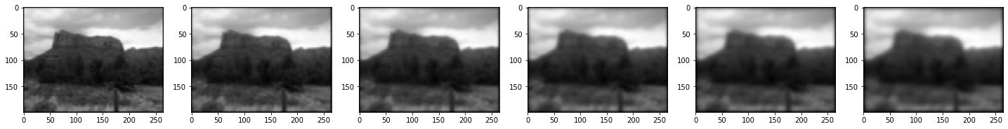
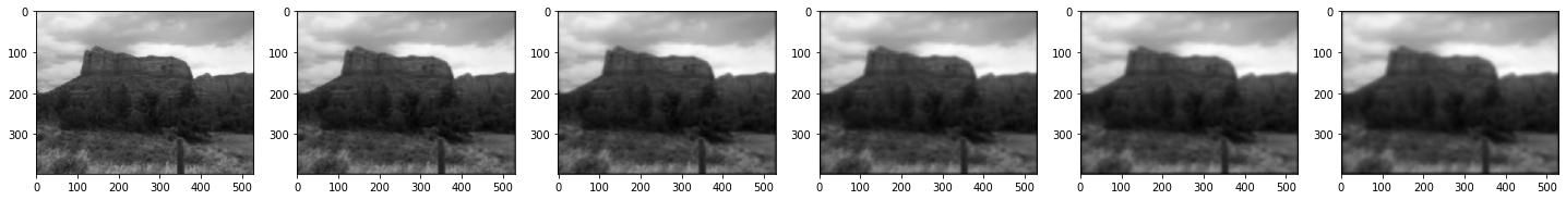
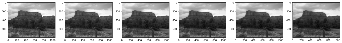
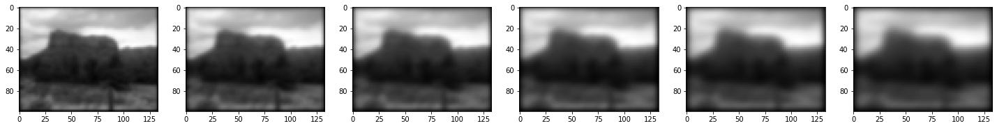
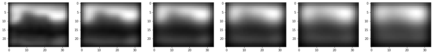
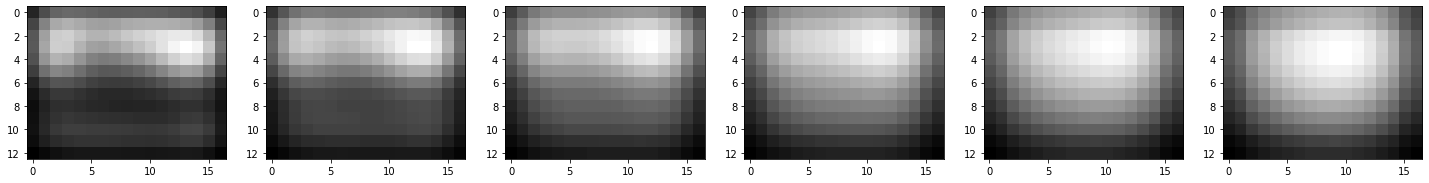
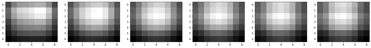
# 显示高斯金字塔图像
gaussian_images = generateGaussianImages(base_image, 8, gaussian_kernels)

for k in range(len(gaussian_images)):
    plt.figure(figsize=(25, 10))
    for i in range(len(gaussian_images[k])):
        plt.subplot(1, len(gaussian_images[k]), i + 1)
        plt.imshow(gaussian_images[k][i].astype(np.uint8), cmap="gray")
plt.show()

[1.6 1.2262735 1.54500779 1.94658784 2.452547 3.09001559]

#################
#生成高斯差分金字塔#
#################
def generateDoGImages(gaussian_images):
    """
    gaussian_images: 传入高斯金字塔组
    """
    # 总的差分金字塔列表
    dog_images = []

    for gaussian_images_in_octave in gaussian_images:
        # 每一组高斯差分金字塔列表
        dog_images_in_octave = []
        # 两两进行差分运算
        for first_image, second_image in zip(gaussian_images_in_octave,
                                             gaussian_images_in_octave[1:]):
            dog_images_in_octave.append(cv2.subtract(
                second_image, first_image))  # 普通的减法不行，因为图像是无符号整数
        dog_images.append(dog_images_in_octave)
    return array(dog_images)

# 显示差分金字塔图像
dog_images = generateDoGImages(gaussian_images)
for k in range(len(dog_images)):
    plt.figure(figsize=(25, 10))
    for i in range(len(dog_images[k])):
        plt.subplot(1, len(dog_images[k]), i + 1)
        plt.imshow(dog_images[k][i].astype(np.uint8), cmap="gray")
plt.show()

####################
#查找极值点的像素位置#
####################
def findScaleSpaceExtrema(gaussian_images,
                          dog_images,
                          num_intervals,
                          sigma,
                          image_border_width,
                          contrast_threshold=0.04):
    """
    gaussian_images: 高斯金字塔组
    dog_images: 差分金字塔组
    num_intervals：每一组极值点检测层数
    sigma：模糊度
    image_border_width：靠近图像边缘5个像素的区域不做检测
    contrast_threshold：对比度阈值
    """
    # 阈值化，不保留低于阈值的不稳定点
    # abs(val)  > 0.5*T/n
    threshold = np.floor(0.5 * contrast_threshold / num_intervals * 255)
    # 关键点列表
    keypoints = []
    # 遍历DoG金字塔
    for octave_index, dog_images_in_octave in enumerate(dog_images):
        # dog_images_in_octave是一个列表，每一个包含5张图片
        # dog_images_in_octave[1:]，包含4张图片
        # dog_images_in_octave[2:]，包含3张图片
        for image_index, (first_image, second_image, third_image) in enumerate(
                zip(dog_images_in_octave, dog_images_in_octave[1:],
                    dog_images_in_octave[2:])):
            # 这里(0,1,2)、(1,2,3)、(2,3,4) 每3张图片分别是一组
            # (i, j) 是3x3矩阵的中心
            # 靠近图像边缘5个像素的区域不做检测,image_border_width=5
            for i in range(image_border_width,
                           first_image.shape[0] - image_border_width):
                for j in range(image_border_width,
                               first_image.shape[1] - image_border_width):
                    ## 调用函数判别极值
                    if isPixelAnExtremum(
                            first_image[i - 1:i + 2, j - 1:j + 2],
                            second_image[i - 1:i + 2, j - 1:j + 2],
                            third_image[i - 1:i + 2, j - 1:j + 2], threshold):
                        ## 调用函数定位极值点（精确定位）
                        localization_result = localizeExtremumViaQuadraticFit(
                            i, j, image_index + 1, octave_index, num_intervals,
                            dog_images_in_octave, sigma, contrast_threshold,
                            image_border_width)
                        if localization_result is not None:
                            keypoint, localized_image_index = localization_result
                            # 计算关键点方向
                            keypoints_with_orientations = computeKeypointsWithOrientations(
                                keypoint, octave_index,
                                gaussian_images[octave_index]
                                [localized_image_index])
                            for keypoint_with_orientation in keypoints_with_orientations:
                                keypoints.append(keypoint_with_orientation)
    return keypoints

#############
#进行极值判别#
#############
def isPixelAnExtremum(first_subimage, second_subimage, third_subimage,
                      threshold):
    """
    first_subimage：第一张图片
    second_subimage：第二张图片
    third_subimage：第三张图片
    threshold：阈值
    满足条件返回True，不满足条件返回False
    """
    center_pixel_value = second_subimage[1, 1]  # 中心像素为第二层中间者
    # 小于阈值的极值点删除
    if abs(center_pixel_value) > threshold:
        if center_pixel_value > 0:
            # 正值情况
            # 分别与上一层9个、下一层9个和本层8个像素进行比较
            return all(center_pixel_value >= first_subimage) and \
                   all(center_pixel_value >= third_subimage) and \
                   all(center_pixel_value >= second_subimage[0, :]) and \
                   all(center_pixel_value >= second_subimage[2, :]) and \
                   center_pixel_value >= second_subimage[1, 0] and \
                   center_pixel_value >= second_subimage[1, 2]
        elif center_pixel_value < 0:
            # 负值情况
            # 分别于上一层9个、一层9个和本层8个像素进行比较
            return all(center_pixel_value <= first_subimage) and \
                   all(center_pixel_value <= third_subimage) and \
                   all(center_pixel_value <= second_subimage[0, :]) and \
                   all(center_pixel_value <= second_subimage[2, :]) and \
                   center_pixel_value <= second_subimage[1, 0] and \
                   center_pixel_value <= second_subimage[1, 2]
    return False

#####################
#二次拟合精确定位极值点#
#####################
def localizeExtremumViaQuadraticFit(i,
                                    j,
                                    image_index,
                                    octave_index,
                                    num_intervals,
                                    dog_images_in_octave,
                                    sigma,
                                    contrast_threshold,
                                    image_border_width,
                                    eigenvalue_ratio=10,
                                    num_attempts_until_convergence=5):
    """
    i，j：中心像素点原坐标
    image_index：每一octave种的图像索引
    octave_index：差分金字塔octave索引
    num_intervals：每一组极值点检测层数
    dog_images_in_octave：高斯差分金字塔组，每一组4张图片
    sigma：高斯模糊度
    contrast_threshold：对比度阈值
    image_border_width：图像边界5像素不检测
    eigenvalue_ratio：主曲率阈值
    num_attempts_until_convergence：最大尝试次数
    """
    extremum_is_outside_image = False
    # 获取每一octave第一层图像尺寸
    image_shape = dog_images_in_octave[0].shape
    # 最大尝试次数设为5
    for attempt_index in range(num_attempts_until_convergence):
        first_image, second_image, third_image = dog_images_in_octave[
            image_index - 1:image_index + 2]
        # 纵向拼接形成三维数组
        pixel_cube = np.stack([
            first_image[i - 1:i + 2, j - 1:j + 2],
            second_image[i - 1:i + 2, j - 1:j + 2], third_image[i - 1:i + 2,
                                                                j - 1:j + 2]
        ]).astype('float32') / 255.
        # 需要从uint8转换为float32以计算导数，并且需要将像素值重新缩放为[0，1]以应用阈值

        # 计算梯度
        gradient = computeGradientAtCenterPixel(pixel_cube)
        # 计算海森阵
        hessian = computeHessianAtCenterPixel(pixel_cube)
        # 最小二乘拟合
        extremum_update = -lstsq(hessian, gradient, rcond=None)[0]
        # 如果当前偏移量绝对值中的每个值均小于0.5，放弃迭代
        if abs(extremum_update[0]) < 0.5 and abs(
                extremum_update[1]) < 0.5 and abs(extremum_update[2]) < 0.5:
            break
        # 更新中心点坐标，即极值点重定位
        j += int(round(extremum_update[0]))
        i += int(round(extremum_update[1]))
        image_index += int(round(extremum_update[2]))
        # 确保新的pixel_cube将完全位于图像中
        if i < image_border_width or i >= image_shape[
                0] - image_border_width or j < image_border_width or j >= image_shape[
                    1] - image_border_width or image_index < 1 or image_index > num_intervals:
            extremum_is_outside_image = True
            break
    if extremum_is_outside_image:
        # 更新的极值在达到收敛之前移出图像
        return None
    if attempt_index >= num_attempts_until_convergence - 1:
        # 超过最大尝试次数，但未达到此极值的收敛。
        return None
    functionValueAtUpdatedExtremum = pixel_cube[1, 1, 1] + 0.5 * np.dot(
        gradient, extremum_update)
    if abs(functionValueAtUpdatedExtremum
           ) * num_intervals >= contrast_threshold:
        xy_hessian = hessian[:2, :2]
        # trace求取xy_hessian的对角元素和
        xy_hessian_trace = trace(xy_hessian)
        # det为求xy_hessian的行列式值
        xy_hessian_det = det(xy_hessian)
        # 检测主曲率是否在域值eigenvalue_ratio下
        if xy_hessian_det > 0 and eigenvalue_ratio * (xy_hessian_trace**2) < (
            (eigenvalue_ratio + 1)**2) * xy_hessian_det:
            # 返回KeyPoint对象,
            keypoint = cv2.KeyPoint()
            # 关键点的点坐标
            keypoint.pt = ((j + extremum_update[0]) * (2**octave_index),
                           (i + extremum_update[1]) * (2**octave_index))
            # 从哪一层金字塔得到的此关键点
            keypoint.octave = octave_index + image_index * (2**8) + int(
                round((extremum_update[2] + 0.5) * 255)) * (2**16)
            # 关键点邻域直径大小
            keypoint.size = sigma * (2**(
                (image_index + extremum_update[2]) / np.float32(num_intervals)
            )) * (2**(octave_index + 1))  # octave_index + 1，因为输入的图像是原来的两倍
            # 响应程度,代表该点的强壮程度,也就是该点角点程度
            keypoint.response = abs(functionValueAtUpdatedExtremum)
            return keypoint, image_index
    return None

##############
#近似求离散梯度#
##############
def computeGradientAtCenterPixel(pixel_array):
    """
    pixel_array：3层3x3的像素区域，进行极值比较
    """
    # 对于步长h，f'(x)的中心差分公式为（f（x + h）-f（x-h））/（2 * h）
    # 此处h = 1，因此公式简化为f'（x）=（f（x + 1）-f（x-1））/ 2

    # x对应于第二个数组轴，y对应于第一个数组轴，s（尺度）对应于第三个数组轴

    dx = 0.5 * (pixel_array[1, 1, 2] - pixel_array[1, 1, 0])
    dy = 0.5 * (pixel_array[1, 2, 1] - pixel_array[1, 0, 1])
    ds = 0.5 * (pixel_array[2, 1, 1] - pixel_array[0, 1, 1])  # 跨层差分
    return np.array([dx, dy, ds])

#############
#近似求海森阵#
#############
def computeHessianAtCenterPixel(pixel_array):
    """
    """
    # 步长为h时，f"(x)的中心差分公式为(f(x+h)-2*f(x)+f(x-h))/(h^2)
    # 这里h= 1，公式化简为f"(x)=f(x+1)-2*f(x)+f(x-1)
    
    # 步长为h时，(d^2)f(x，y)/(dxdy）的中心差分公式为：
    # (f(x+h，y+h)-f(x+h，y-h)-f(x-h，y+h)+ f(x-h，y-h))/(4*h^2)
    # 在这里h = 1，因此公式简化为：
    # (d^2)f(x，y)/(dx dy)=(f(x+1，y+1)-f(x+1，y-1)-f(x-1，y+1)+f(x-1，y-1))/4
    
    # x对应于第二个数组轴，y对应于第一个数组轴，s（尺度）对应于第三个数组轴
    center_pixel_value = pixel_array[1, 1, 1] # 中心像素值
    dxx = pixel_array[1, 1, 2] - 2 * center_pixel_value + pixel_array[1, 1, 0]
    dyy = pixel_array[1, 2, 1] - 2 * center_pixel_value + pixel_array[1, 0, 1]
    dss = pixel_array[2, 1, 1] - 2 * center_pixel_value + pixel_array[0, 1, 1]
    dxy = 0.25 * (pixel_array[1, 2, 2] - pixel_array[1, 2, 0] -
                  pixel_array[1, 0, 2] + pixel_array[1, 0, 0])
    dxs = 0.25 * (pixel_array[2, 1, 2] - pixel_array[2, 1, 0] -
                  pixel_array[0, 1, 2] + pixel_array[0, 1, 0])
    dys = 0.25 * (pixel_array[2, 2, 1] - pixel_array[2, 0, 1] -
                  pixel_array[0, 2, 1] + pixel_array[0, 0, 1])
    return np.array([[dxx, dxy, dxs], [dxy, dyy, dys], [dxs, dys, dss]])

###############################
##########计算关键点方向#########
#为关键点附近的像素创建渐变的直方图#
###############################
def computeKeypointsWithOrientations(keypoint,
                                     octave_index,
                                     gaussian_image,
                                     radius_factor=3,
                                     num_bins=36,
                                     peak_ratio=0.8,
                                     scale_factor=1.5):
    """
    keypoint：检测到精确并定位的关键点
    octave_index：差分金字塔octave索引
    gaussian_image：高斯金字塔组
    radius_factor：半径因子
    num_bins：直方图柱数，没0度一柱
    peak_ratio：只保留峰值大于主方向峰值80％的方向作为该关键点的辅方向
    scale_factor：尺度因子
    """
    keypoints_with_orientations = []
    image_shape = gaussian_image.shape

    # scale = 1.5*sigma
    scale = scale_factor * keypoint.size / np.float32(2**(octave_index + 1))
    # 直方图统计半径采用3*1.5*sigma
    radius = int(round(radius_factor * scale))
    # 权重因子
    weight_factor = -0.5 / (scale**2)
    # 梯度直方图将0~360度的方向范围分为36个柱(bins)，其中每柱10度
    # num_bins=36
    raw_histogram = np.zeros(num_bins)
    # 高斯平滑直方图
    smooth_histogram = np.zeros(num_bins)

    # 采集其所在高斯金字塔图像3σ领域窗口内像素的梯度和方向分布特征
    for i in range(-radius, radius + 1):
        region_y = int(round(keypoint.pt[1] / np.float32(2**octave_index))) + i
        if region_y > 0 and region_y < image_shape[0] - 1:
            for j in range(-radius, radius + 1):
                region_x = int(
                    round(keypoint.pt[0] / np.float32(2**octave_index))) + j
                if region_x > 0 and region_x < image_shape[1] - 1:
                    # 差分求偏导，这里省略了1/2的系数
                    dx = gaussian_image[region_y, region_x +
                                        1] - gaussian_image[region_y,
                                                            region_x - 1]
                    dy = gaussian_image[region_y - 1,
                                        region_x] - gaussian_image[region_y +
                                                                   1, region_x]
                    # 梯度模值
                    gradient_magnitude = np.sqrt(dx * dx + dy * dy)
                    # 梯度方向
                    gradient_orientation = np.rad2deg(np.arctan2(dy, dx))
                    weight = np.exp(weight_factor * (i**2 + j**2))
                    # 梯度幅值需先乘以高斯权重再累加到直方图中去
                    histogram_index = int(
                        round(gradient_orientation * num_bins / 360.))
                    raw_histogram[histogram_index %
                                  num_bins] += weight * gradient_magnitude

    for n in range(num_bins):
        # 使用平滑公式
        smooth_histogram[n] = (
            6 * raw_histogram[n] + 4 *
            (raw_histogram[n - 1] + raw_histogram[(n + 1) % num_bins]) +
            raw_histogram[n - 2] + raw_histogram[(n + 2) % num_bins]) / 16.
    orientation_max = max(smooth_histogram)
    # 找出主方向
    orientation_peaks = where(
        np.logical_and(smooth_histogram > roll(smooth_histogram, 1),
                       smooth_histogram > roll(smooth_histogram, -1)))[0]
    for peak_index in orientation_peaks:
        peak_value = smooth_histogram[peak_index]
        # 辅方向，阈值为80%
        if peak_value >= peak_ratio * orientation_max:
            left_value = smooth_histogram[(peak_index - 1) % num_bins]
            right_value = smooth_histogram[(peak_index + 1) % num_bins]
            # 梯度直方图抛物线插值
            interpolated_peak_index = (
                peak_index + 0.5 * (left_value - right_value) /
                (left_value - 2 * peak_value + right_value)) % num_bins
            orientation = 360. - interpolated_peak_index * 360. / num_bins
            if abs(orientation - 360.) < float_tolerance:
                orientation = 0
            new_keypoint = cv2.KeyPoint(*keypoint.pt, keypoint.size,
                                        orientation, keypoint.response,
                                        keypoint.octave)
            keypoints_with_orientations.append(new_keypoint)
    return keypoints_with_orientations

################
#对关键点进行比较#
################
def compareKeypoints(keypoint1, keypoint2):
    """
    keypoint1、keypoint2：需要比较的两个关键点
    """
    # 关键点的点坐标
    if keypoint1.pt[0] != keypoint2.pt[0]:
        return keypoint1.pt[0] - keypoint2.pt[0]
    if keypoint1.pt[1] != keypoint2.pt[1]:
        return keypoint1.pt[1] - keypoint2.pt[1]
    # 关键点邻域直径大小
    if keypoint1.size != keypoint2.size:
        return keypoint2.size - keypoint1.size
    # 角度，表示关键点的方向，值为[零,三百六十)，负值表示不使用
    if keypoint1.angle != keypoint2.angle:
        return keypoint1.angle - keypoint2.angle
    # 响应强度
    if keypoint1.response != keypoint2.response:
        return keypoint2.response - keypoint1.response
    # 从哪一层金字塔得到的此关键点
    if keypoint1.octave != keypoint2.octave:
        return keypoint2.octave - keypoint1.octave
    return keypoint2.class_id - keypoint1.class_id

################
#排序并删除重复项#
################
def removeDuplicateKeypoints(keypoints):
    """
    keypoints：关键点
    """
    if len(keypoints) < 2:
        return keypoints
    # 进行排序
    keypoints.sort(key=cmp_to_key(compareKeypoints))
    unique_keypoints = [keypoints[0]]
    # 删除重复值
    for next_keypoint in keypoints[1:]:
        last_unique_keypoint = unique_keypoints[-1]
        if last_unique_keypoint.pt[0] != next_keypoint.pt[0] or \
           last_unique_keypoint.pt[1] != next_keypoint.pt[1] or \
           last_unique_keypoint.size != next_keypoint.size or \
           last_unique_keypoint.angle != next_keypoint.angle:
            unique_keypoints.append(next_keypoint)
    return unique_keypoints

####################################
#将关键点从基本图像坐标转换为输入图像坐标#
####################################
def convertKeypointsToInputImageSize(keypoints):
    """
    keypoints：关键点
    """
    converted_keypoints = []
    for keypoint in keypoints:
        keypoint.pt = tuple(0.5 * np.array(keypoint.pt))
        keypoint.size *= 0.5
        keypoint.octave = (keypoint.octave & ~255) | (
            (keypoint.octave - 1) & 255)
        converted_keypoints.append(keypoint)
    return converted_keypoints

#############
#“解压”关键点#
############
def unpackOctave(keypoint):
    """
    计算每一个关键点的octave、layer和scale
    """
    octave = keypoint.octave & 255
    layer = (keypoint.octave >> 8) & 255
    if octave >= 128:
        octave = octave | -128
    scale = 1 / np.float32(1 << octave) if octave >= 0 else np.float32(
        1 << -octave)
    return octave, layer, scale

####################
#为每个关键点生成描述符#
####################
def generateDescriptors(keypoints,
                        gaussian_images,
                        window_width=4,
                        num_bins=8,
                        scale_multiplier=3,
                        descriptor_max_value=0.2):
    """
    keypoints：关键点
    gaussian_images：高斯金字塔图像
    window_width：关键点附近的区域长为4，4X4个子区域
    num_bins：8个方向的梯度直方图
    scale_multiplier：
    descriptor_max_value：
    """
    descriptors = []

    for keypoint in keypoints:
        # 进行“解压缩”
        octave, layer, scale = unpackOctave(keypoint)
        # 关键点所对应的高斯金字塔图像
        gaussian_image = gaussian_images[octave + 1, layer]
        # 该图像的尺寸
        num_rows, num_cols = gaussian_image.shape
        # 定位
        point = np.round(scale * np.array(keypoint.pt)).astype('int')
        # 为方便后面计算的变量
        bins_per_degree = num_bins / 360.
        # 为方便后面旋转
        angle = 360. - keypoint.angle
        cos_angle = np.cos(deg2rad(angle))  # 角度转弧度
        sin_angle = np.sin(deg2rad(angle))  # 角度转弧度
        # Lowe 建议子区域的像素的梯度大小按0.5d的高斯加权计算
        weight_multiplier = -0.5 / ((0.5 * window_width)**2)
        row_bin_list = []
        col_bin_list = []
        magnitude_list = []
        orientation_bin_list = []
        histogram_tensor = np.zeros(
            (window_width + 2, window_width + 2, num_bins))  # 前两个维度增加2
        # 把3sigma长度作为一个单元长度
        hist_width = scale_multiplier * 0.5 * scale * keypoint.size
        # 实际计算所需的图像区域半径（根据公式）
        # 说明一下，这里就是一个大圆外套一个正方形
        half_width = int(
            np.round(hist_width * np.sqrt(2) * (window_width + 1) *
                     0.5))  # sqrt(2)对应于像素的对角线长度
        # 最终区域长度
        half_width = int(min(half_width, sqrt(num_rows**2 + num_cols**2)))

        # 坐标轴旋转至主方向
        for row in range(-half_width, half_width + 1):
            for col in range(-half_width, half_width + 1):
                row_rot = col * sin_angle + row * cos_angle  # 旋转后的特征点坐标
                col_rot = col * cos_angle - row * sin_angle  # 旋转后的特征点坐标
                # 计算旋转后的特征点落在子区域的下标
                # 坐标归一化
                # +（d/2）是把坐标系由特征点处平移至左上角的边界点
                # -0.5则是回移坐标系至描述子区间中的第一个子区间的中心处
                row_bin = (row_rot / hist_width) + 0.5 * window_width - 0.5
                col_bin = (col_rot / hist_width) + 0.5 * window_width - 0.5
               
                if row_bin > -1 and row_bin < window_width and col_bin > -1 and col_bin < window_width:
                    window_row = int(np.round(point[1] + row))
                    window_col = int(np.round(point[0] + col))
                    if window_row > 0 and window_row < num_rows - 1 and window_col > 0 and window_col < num_cols - 1:
                        # 求偏导
                        dx = gaussian_image[window_row, window_col +
                                            1] - gaussian_image[window_row,
                                                                window_col - 1]
                        dy = gaussian_image[window_row - 1,
                                            window_col] - gaussian_image[
                                                window_row + 1, window_col]
                        # 模值
                        gradient_magnitude = np.sqrt(dx * dx + dy * dy)
                        # 方向
                        gradient_orientation = np.rad2deg(arctan2(dy,
                                                                  dx)) % 360
                        # 高斯加权值
                        weight = np.exp(weight_multiplier *
                                        ((row_rot / hist_width)**2 +
                                         (col_rot / hist_width)**2))
                        
                        row_bin_list.append(row_bin)
                        col_bin_list.append(col_bin)
                        magnitude_list.append(weight * gradient_magnitude)
                        orientation_bin_list.append(
                            (gradient_orientation - angle) * bins_per_degree)

        for row_bin, col_bin, magnitude, orientation_bin in zip(
                row_bin_list, col_bin_list, magnitude_list,
                orientation_bin_list):
            # 通过三线性插值平滑
            # 实际上是在做三线性插值的逆(取立方体的中心值，并将其分配给它的八个邻域)
            row_bin_floor, col_bin_floor, orientation_bin_floor = floor(
                [row_bin, col_bin, orientation_bin]).astype(int)
            # 计算差值部分，小数余项
            row_fraction, col_fraction, orientation_fraction = row_bin - row_bin_floor, col_bin - col_bin_floor, orientation_bin - orientation_bin_floor
            if orientation_bin_floor < 0:
                orientation_bin_floor += num_bins
            if orientation_bin_floor >= num_bins:
                orientation_bin_floor -= num_bins

            c1 = magnitude * row_fraction
            c0 = magnitude * (1 - row_fraction)
            
            c11 = c1 * col_fraction
            c10 = c1 * (1 - col_fraction)
            c01 = c0 * col_fraction
            c00 = c0 * (1 - col_fraction)
            # 最终累加在每个方向上的梯度大小为
            c111 = c11 * orientation_fraction
            c110 = c11 * (1 - orientation_fraction)
            c101 = c10 * orientation_fraction
            c100 = c10 * (1 - orientation_fraction)
            c011 = c01 * orientation_fraction
            c010 = c01 * (1 - orientation_fraction)
            c001 = c00 * orientation_fraction
            c000 = c00 * (1 - orientation_fraction)

            histogram_tensor[row_bin_floor + 1, col_bin_floor + 1,
                             orientation_bin_floor] += c000
            histogram_tensor[row_bin_floor + 1, col_bin_floor + 1,
                             (orientation_bin_floor + 1) % num_bins] += c001
            histogram_tensor[row_bin_floor + 1, col_bin_floor + 2,
                             orientation_bin_floor] += c010
            histogram_tensor[row_bin_floor + 1, col_bin_floor + 2,
                             (orientation_bin_floor + 1) % num_bins] += c011
            histogram_tensor[row_bin_floor + 2, col_bin_floor + 1,
                             orientation_bin_floor] += c100
            histogram_tensor[row_bin_floor + 2, col_bin_floor + 1,
                             (orientation_bin_floor + 1) % num_bins] += c101
            histogram_tensor[row_bin_floor + 2, col_bin_floor + 2,
                             orientation_bin_floor] += c110
            histogram_tensor[row_bin_floor + 2, col_bin_floor + 2,
                             (orientation_bin_floor + 1) % num_bins] += c111

        descriptor_vector = histogram_tensor[1:-1,
                                             1:-1, :].flatten()  # 删除直方图边界
        # 设定阈值，并归一化描述符
        threshold = norm(descriptor_vector) * descriptor_max_value
        descriptor_vector[descriptor_vector > threshold] = threshold
        descriptor_vector /= max(norm(descriptor_vector), float_tolerance)

        descriptor_vector = np.round(512 * descriptor_vector)
        descriptor_vector[descriptor_vector < 0] = 0
        descriptor_vector[descriptor_vector > 255] = 255
        descriptors.append(descriptor_vector)

    return array(descriptors, dtype='float32')

##########主函数###############
##############################
#计算输入图像的SIFT关键点和描述符#
##############################
def computeKeypointsAndDescriptors(image,
                                   sigma=1.6,
                                   num_intervals=3,
                                   assumed_blur=0.5,
                                   image_border_width=5):
    """
    image：输入图像
    sigma：目标高斯模糊度
    num_intervals：能进行极值点检测的图层数
    assumed_blur：假设模糊度
    image_border_width：图像边缘5个像素不检测
    """
    image = image.astype(np.float32)
    # 升采样生成基图像（为了尽可能多地保留原始图像信息，对原始图像进行扩大两倍采样）
    base_image = generateBaseImage(image, sigma, assumed_blur)
    # 计算可以将图像重复减半直到变得很小的次数
    num_octaves = computeNumberOfOctaves(base_image.shape)
    # 生成高斯模糊度列表，以产生尺度金字塔
    gaussian_kernels = generateGaussianKernels(sigma, num_intervals)
    # 生成高斯金字塔
    gaussian_images = generateGaussianImages(base_image, num_octaves,
                                             gaussian_kernels)
    # 生成高斯差分金字塔
    dog_images = generateDoGImages(gaussian_images)
    # 寻找关键点
    keypoints = findScaleSpaceExtrema(gaussian_images, dog_images,
                                      num_intervals, sigma, image_border_width)
    # 对关键点进行去重处理
    keypoints = removeDuplicateKeypoints(keypoints)
    # 将关键点从基本图像坐标转换为输入图像坐标
    keypoints = convertKeypointsToInputImageSize(keypoints)
    # 为关键点生成描述符
    descriptors = generateDescriptors(keypoints, gaussian_images)
    return keypoints, descriptors

kp1, des1 = computeKeypointsAndDescriptors(img1)
# 左图特征点可视化
fig = plt.figure()
ax =fig.add_subplot(111)
plt.imshow(img1, cmap='gray')
for i in range(len(kp1)):
   ax.plot(kp1[i].pt[0], kp1[i].pt[1], '.', color = 'red')
plt.show()

kp2, des2 = computeKeypointsAndDescriptors(img2)
# 右图特征点可视化
fig = plt.figure()
ax =fig.add_subplot(111)
plt.imshow(img2, cmap='gray')
for i in range(len(kp2)):
   ax.plot(kp2[i].pt[0], kp2[i].pt[1], '.', color = 'blue')

imageA = img2 # 右图
imageB = img1 # 左图
kpsA = kp2
kpsB = kp1 # 特征点
featuresA = des2
featuresB = des1 # 特征向量
kpsA = np.float32([kp.pt for kp in kpsA]) # 类型转换
kpsB = np.float32([kp.pt for kp in kpsB])

###########
#全景图生成#
##########
class Stitcher:
    # 拼接函数
    def stitch(self, images, ratio=0.75, reprojThresh=4.0, showMatches=False):
        # 获取输入图片
        (imageA, imageB) = images

        # 匹配两张图片的所有特征点，返回匹配结果
        M = self.matchKeypoints(kpsA, kpsB, featuresA, featuresB, ratio,
                                reprojThresh)

        # 如果返回结果为空，没有匹配成功的特征点，退出算法
        if M is None:
            return None

        # 否则，提取匹配结果
        # H是3x3视角变换矩阵
        (matches, H, status) = M
        # 将图片A进行视角变换，result是变换后图片
        result = cv2.warpPerspective(
            imageA, H, (imageA.shape[1] + imageB.shape[1], imageA.shape[0]))
        self.cv_show('result', result)
        # 将图片B传入result图片最左端
        result[0:imageB.shape[0], 0:imageB.shape[1]] = imageB
        self.cv_show('result', result)
        # 检测是否需要显示图片匹配
        if showMatches:
            # 生成匹配图片
            vis = self.drawMatches(imageA, imageB, kpsA, kpsB, matches, status)
            # 返回结果
            return (result, vis)

        # 返回匹配结果
        return result

    def cv_show(self, name, img):
        cv2.imshow(name, img)
        cv2.waitKey(0)
        cv2.destroyAllWindows()

    def matchKeypoints(self, kpsA, kpsB, featuresA, featuresB, ratio,
                       reprojThresh):
        # 建立暴力匹配器
        matcher = cv2.BFMatcher()
        
        # 使用KNN检测来自A、B图的SIFT特征匹配对，K=2
        rawMatches = matcher.knnMatch(featuresA, featuresB, 2)  # 检测出每个点，匹配的2个点
        # 返回的M结果为[(1, 6), ..,(112, 113)]等等，里面的数字为第几个特征点
        matches = []
        for m in rawMatches:
            # 当最近距离跟次近距离的比值小于ratio值时，保留此匹配对
            if len(m) == 2 and m[0].distance < m[1].distance * ratio:
                # 存储两个点在featuresA, featuresB中的索引值
                matches.append((m[0].trainIdx, m[0].queryIdx))

        # 当筛选后的匹配对大于4时，计算视角变换矩阵
        if len(matches) > 4:
            # 获取匹配对的点坐标（float32型）
            ptsA = np.float32([kpsA[i] for (_, i) in matches])
            print(ptsA.shape)  # (148, 2)
            ptsB = np.float32([kpsB[i] for (i, _) in matches])

            # 计算视角变换矩阵（把RANSAC和计算H矩阵合并到了一起）
            (H, status) = cv2.findHomography(ptsA, ptsB, cv2.RANSAC,
                                             reprojThresh)
            # 该函数的作用就是先用RANSAC选择最优的四组配对点，再计算H矩阵。H为3*3矩阵
            print(status.shape)
            # 返回结果
            return (matches, H, status)

        # 如果匹配对小于4时，返回None
        return None

    def drawMatches(self, imageA, imageB, kpsA, kpsB, matches, status):
        # 初始化可视化图片，将A、B图左右连接到一起
        (hA, wA) = imageA.shape
        (hB, wB) = imageB.shape
        vis = np.zeros((max(hA, hB), wA + wB), dtype="uint8")
        vis[0:hA, 0:wA] = imageA
        vis[0:hB, wA:] = imageB

        # 联合遍历，画出匹配对
        for ((trainIdx, queryIdx), s) in zip(matches, status):
            # 当点对匹配成功时，画到可视化图上
            if s == 1:
                # 画出匹配对
                ptA = (int(kpsA[queryIdx][0]), int(kpsA[queryIdx][1]))
                ptB = (int(kpsB[trainIdx][0]) + wA, int(kpsB[trainIdx][1]))
                cv2.circle(vis, ptA, 5, (0, 0, 255), 1)
                cv2.circle(vis, ptB, 5, (0, 0, 255), 1)
                cv2.line(vis, ptA, ptB, (0, 0, 255), 1)

        # 返回可视化结果
        return vis

# 对右边的图形做变换
# 把图片拼接成全景图
stitcher = Stitcher()
(result, vis) = stitcher.stitch([imageA, imageB], showMatches=True)

# 显示所有图片
cv2.imshow("Image A", imageA)
cv2.imshow("Image B", imageB)
cv2.imshow("Keypoint Matches", vis)
cv2.imshow("Result", result)
cv2.waitKey(0)
cv2.destroyAllWindows()

完整代码我已放到我的资源下载中心，田纳尔多，可以在上面下载。

4 实验结果与分析

1、原始图像

左图	右图

2、两张图像的特征点匹配

在这里插入图片描述

3、右图作了变形的结果

在这里插入图片描述

4、拼接结果

在这里插入图片描述

可以看出两张图片已经被连接在了一起，图片间没有明显的分割与错位，整体上也没有照片之间的独立感。连续的拼接需要右侧的图像不断被仿射变化来与左侧图像连接，而导致了最右侧的图像在最终的全景图中有些扭曲。整体来说，还算成功！