无人驾驶汽车系统入门（三十）——基于深度神经网络LaneNet的车道线检测及ROS实现

无人驾驶汽车系统入门（三十）——基于深度神经网络LaneNet的车道线检测及ROS实现

前面的博文介绍了基于传统视觉的车道线检测方法，传统视觉车道线检测方法主要分为提取特征、车道像素聚类和车道线多项式拟合三个步骤。然而，无论是颜色特征还是梯度特征，人为设计的特征阈值存在鲁棒性差的问题，深度学习方法为车道线的检测带来了高鲁棒性的解决思路，在近年来逐步替代了传统视觉方法，本文介绍一种用于车道线检测的典型神经网络LaneNet，并且基于其开源的实现代码编写了一个ROS程序。

论文原文地址：Towards End-to-End Lane Detection: an Instance Segmentation Approach

Tensorflow实现代码原地址：lanenet-lane-detection

本文ROS实现代码地址：LaneNetRos

如果你想在Python2环境下训练LaneNet，试试我修改的版本：lanenet-lane-detection-py2

LaneNet 网络结构

LaneNet将图像中的车道线检测看作是一个实例分割（Instance Segmentation）问题，是一个端到端的模型，输入图像，网络直接输出车道线像素以及每个像素对应的车道线ID，无需人为设计特征，在提取出车道像素以及车道ID以后，通常我们将图像投射到鸟瞰视角，以进一步完成车道线拟合（主要是三次多项式拟合），传统的做法是使用一个固定的变换矩阵对图像进行透视变换，这种方法在路面不平的情况下存在较大的偏差，而论文作者的做法是训练一个名为H-Net的简单神经网络，输入当前图像到H-Net，这个简单神经网络输出相应的鸟瞰变换矩阵。完成鸟瞰变换以后，使用最小二乘法拟合一个2次（或者3次）多项式，从而完成车道线检测。

如上图是LaneNet的网络结构，和传统的语义分割网络类似，包含编码网络（Encoder）和解码网络（Decoder），解码网络包含两个分支，对应的是两类分割：

• 嵌入分支（Embedding branch）：主要用于车道线的实例分割，如图所示，该网络解码得到的输出图中每一个像素对应一个N维的向量，在该N维嵌入空间中同一车道线的像素距离更接近，而不同车道线的像素的向量距离较大，从而区分像素属于哪一条车道线，该分支使用基于one-shot的方法做距离度量学习。
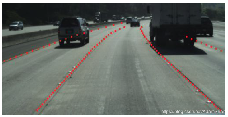
• 分割分支（Segmentation branch）：主要用于获取车道像素的分割结果（得到一个二分图，即筛选出车道线像素和非车道线像素），得到一个二分图像，如上图所示。为了训练一个这样的分割网络，原论文使用了tuSample数据集，在数据集中，车道线可能被其他车辆阻挡，在这种情况下，将车道线的标注(Ground truth)贯穿障碍物，如下图所示，从而使得分割网络在车道线被其他障碍物阻挡的情况下，依然可以完整检测出完整的车道线像素。分割网络使用标准的交叉熵损失函数进行训练，对于这个逐像素分类任务而言（车道线像素/非车道线像素分类），由于两个类别的像素极度不均衡，为了处理此问题，作者使用了bounded inverse class weighting方法（详见论文）。

那么通过叠加嵌入分支和分割分支，在使用神经网络提取出车道线像素的同时，还能够对每个车道线实现聚类（即像素属于哪一根车道线）。为了训练这样的聚类嵌入网络，聚类损失函数（嵌入网络）包含两部分，方差项 $L_{var}$ 和距离项 $L_{dist}$ ,其中 $L_{var}$ 将每个嵌入的向量往某条车道线聚类中心（均值）方向拉，这种“拉力”激活的前提是嵌入向量到平均嵌入向量的距离过远，大于阈值 $\delta_v$ ； $L_{dist}$ 使两个类别的车道线越远越好，激活这个“推力”的前提是两条车道线聚类中心的距离过近，近于阈值 $\delta_d$ 。最后总的损失函数L的公式如下：

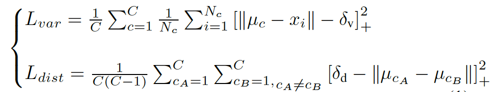
其中 $C$ 表示聚类的数量（也就是车道线的数量）， $N_c$ 表示聚类 $c$ 中的元素数量， $x_i$ 表示一个像素嵌入向量， $\mu_{c}$ 表示聚类 $c$ 的均值向量， $[x]_{+} = max(0, x)$，最后的损失函数为 $L = L_{var} + L_{dist}$ 。该损失函数在实际实现（TensorFlow）中代码如下：

def discriminative_loss_single(
        prediction,
        correct_label,
        feature_dim,
        label_shape,
        delta_v,
        delta_d,
        param_var,
        param_dist,
        param_reg):
    """
    实例分割损失函数
    :param prediction: inference of network
    :param correct_label: instance label
    :param feature_dim: feature dimension of prediction
    :param label_shape: shape of label
    :param delta_v: cut off variance distance
    :param delta_d: cut off cluster distance
    :param param_var: weight for intra cluster variance
    :param param_dist: weight for inter cluster distances
    :param param_reg: weight regularization
    """

    # 像素对齐为一行
    correct_label = tf.reshape(
        correct_label, [
            label_shape[1] * label_shape[0]])
    reshaped_pred = tf.reshape(
        prediction, [
            label_shape[1] * label_shape[0], feature_dim])

    # 统计实例个数
    unique_labels, unique_id, counts = tf.unique_with_counts(correct_label)
    counts = tf.cast(counts, tf.float32)
    num_instances = tf.size(unique_labels)

    # 计算pixel embedding均值向量
    segmented_sum = tf.unsorted_segment_sum(
        reshaped_pred, unique_id, num_instances)
    mu = tf.div(segmented_sum, tf.reshape(counts, (-1, 1)))
    mu_expand = tf.gather(mu, unique_id)

    # 计算公式的loss(var)
    distance = tf.norm(tf.subtract(mu_expand, reshaped_pred), axis=1)
    distance = tf.subtract(distance, delta_v)
    distance = tf.clip_by_value(distance, 0., distance)
    distance = tf.square(distance)

    l_var = tf.unsorted_segment_sum(distance, unique_id, num_instances)
    l_var = tf.div(l_var, counts)
    l_var = tf.reduce_sum(l_var)
    l_var = tf.divide(l_var, tf.cast(num_instances, tf.float32))

    # 计算公式的loss(dist)
    mu_interleaved_rep = tf.tile(mu, [num_instances, 1])
    mu_band_rep = tf.tile(mu, [1, num_instances])
    mu_band_rep = tf.reshape(
        mu_band_rep,
        (num_instances *
         num_instances,
         feature_dim))

    mu_diff = tf.subtract(mu_band_rep, mu_interleaved_rep)

    # 去除掩模上的零点
    intermediate_tensor = tf.reduce_sum(tf.abs(mu_diff), axis=1)
    zero_vector = tf.zeros(1, dtype=tf.float32)
    bool_mask = tf.not_equal(intermediate_tensor, zero_vector)
    mu_diff_bool = tf.boolean_mask(mu_diff, bool_mask)

    mu_norm = tf.norm(mu_diff_bool, axis=1)
    mu_norm = tf.subtract(2. * delta_d, mu_norm)
    mu_norm = tf.clip_by_value(mu_norm, 0., mu_norm)
    mu_norm = tf.square(mu_norm)

    l_dist = tf.reduce_mean(mu_norm)

    # 计算原始Discriminative Loss论文中提到的正则项损失
    l_reg = tf.reduce_mean(tf.norm(mu, axis=1))

    # 合并损失按照原始Discriminative Loss论文中提到的参数合并
    param_scale = 1.
    l_var = param_var * l_var
    l_dist = param_dist * l_dist
    l_reg = param_reg * l_reg

    loss = param_scale * (l_var + l_dist + l_reg)

    return loss, l_var, l_dist, l_reg

在上述代码中，首先统计了聚类的个数num_instances （即 $C$ ） 和每个聚类中像素的数量 counts（即 $N_c$ ）。然后计算所有聚类的嵌入向量的均值 mu_expand （即 $\mu_c$），接着按照上述公式计算了 $L_{var}$ （这里 tf.norm 默认采用欧几里得范数，和论文一致）， 同理计算 $L_{dist}$ ，有了这个loss函数，当网络训练收敛，车道线像素的嵌入向量将自动聚类。

在推理（inference）阶段，为了将像素进行聚类，在上述的实例分割损失函数中设置 $\delta_d > 6\delta_v$ 。聚类时，首先使用mean shift聚类，使得簇中心沿着密度上升的方向移动，防止将离群点选入相同的簇中；之后对像素向量进行划分：以簇中心为圆心，以 $2\delta_v$为半径，选取圆中所有的像素归为同一车道线。重复该步骤，直到将所有的车道线像素分配给对应的车道。

编码解码网络结构原论文作者采用的是ENet的结构，实际上编码解码器网络并没有严格的要求（不是非用ENet不可），本例采用的开源实现使用了VGG-16作为编码器，使用了FCN作为解码器网络（本质上就是一个FCN-VGG16语义分割模型），并且使用FCN-8s的跳层策略（即组合第3，4，5个池化层的上采样结果作为最终的预测输出图）实现边缘精炼，这些我们会在后面的代码中具体介绍。

扫描二维码关注公众号，回复： 11402078 查看本文章

H-Net 和 曲线拟合

LaneNet 网络的输出实际上就是各个车道线像素点的，并且知道每个像素属于第几条车道线，接下来就是使用多项式拟合这些像素，得到结构化的车道线检测结果，传统的一个做法就是使用固定的变换矩阵将图像投射到鸟瞰视角，在鸟瞰视角下使用二次或者三次多项式拟合各个车道线，这种方法对于起伏的路面效果不会特别准确，所以原论文作者设计了H-Net来根据图像端到端学习一个变换矩阵，最终输出的变换矩阵有六个自由度，如下：

$H = \begin{bmatrix}a&b&c\\0&d&e\\0&f&1\end{bmatrix}$

H-Net是一个简单的卷积神经网络，其结构如下表所示：

那么经过一轮前向传播，H-Net可以得到一个变换矩阵 $H$ ，为了计算损失，给定包含 $N$ 个车道线像素点ground truth集合 $t_i = [x_{i}, y_{i}, 1]^T \in T$，通过变换矩阵 $H$ 获得转换后的点的集合：

$T' = HT$

其中 $t_i' = [x_i', y_i', 1]^T \in T'$ ，如下图所示：

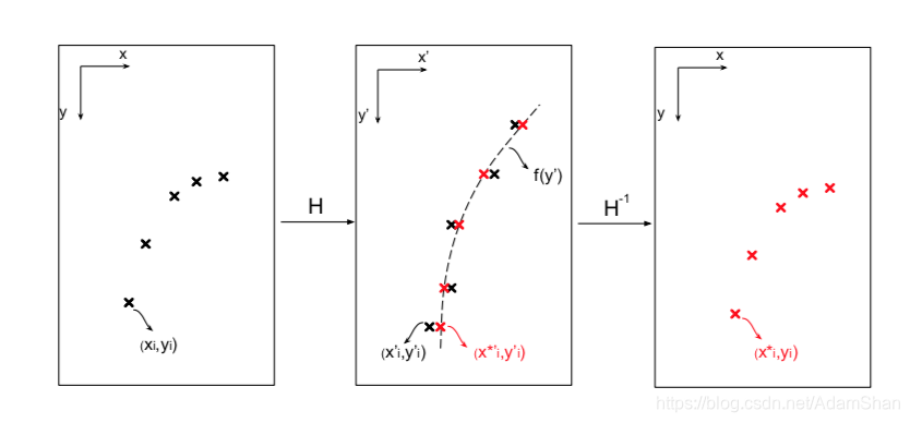
要计算loss，首先要计算ground truth的拟合多项式参数（真实的车道线拟合多项式），论文作者计算二次多项式 $f(y') = \alpha y'^2 + \beta y' + \gamma$ 以拟合所有车道像素点，即求参数向量 $w = (\alpha, \beta, \gamma)^T$ ，论文作者使用最小二乘法实现多项式拟合（最小二乘法曲线拟合详细推导可以参考 该文 ），则参数向量 $w$ 为：

$w = (Y^TY)^{-1}Y^TX$

其中 $X =[x_1', x_2', ..., x_N']^T$ ， $Y = \begin{bmatrix}y_1'^2&y_1'&1\\...&...&...\\y_N'^2&y_N'&1\end{bmatrix}$ ，至此我们就算得了真实车道线的二次多项式。

那么对于LaneNet输出的预测像素 $p_i = [x_{i}, y_{i}, 1]^T \in P$，通过H-Net映射可以得到变换后的像素 $P' = HP$ ，其中 $p_i = [x_i', y_i', 1]^T \in P'$ ， 那么根据 $y_i'$ 就可以根据多项式 $f(y_i')$ 可以计算出 $x_i'^{*}$ , 可以得到向量 $p'^{*} = [x_i'^{*}, y_i']^T$ ，使用变换矩阵反向得到在原图中的点 $p_i^{*} = [x_i^{*}, y_i, 1]^T$ ，那么H-Net的损失函数 $Loss$ 被表示为：

$Loss = \frac{1}{N}\sum_{i=1}^N(x_i^{*} - x_i)^2$

使用该损失函数，H-Net将被学习以产生适配当前图像的变换矩阵。

TensorFlow实现及基于tuSimple数据集的模型训练

数据准备和tfrecord生成

借鉴lanenet-lane-detection项目，我们来分析一下该模型的TensorFlow实现，首先是数据的准备，下载tuSimple数据集(可能需要科学上网)：

• tuSimple训练集下载地址
• tuSimple测试集下载地址

下载完成后解压缩到一个目录下，目录内容如下：

tuSimple/
├── clips
│   ├── 0313-1
│   ├── 0313-2
│   ├── 0530
│   ├── 0531
│   └── 0601
├── label_data_0313.json
├── label_data_0531.json
├── label_data_0601.json
├── readme.md
└── test_tasks_0627.json

我们使用项目lanenet-lane-detection中的脚本generate_tusimple_dataset.py产生用于训练的binary mask和instance mask：

cd lanenet-lane-detection/tools
python3 generate_tusimple_dataset.py --src_dir=/home/adam/data/tusimple_dataset/tuSimple/

如上所示，会自动在tuSimple目录下生成training和testing两个目录，如下所示：

training/
├── gt_binary_image
├── gt_image
├── gt_instance_image
├── label_data_0313.json
├── label_data_0531.json
├── label_data_0601.json
└── train.txt
testing/
└── test_tasks_0627.json

可见该脚本仅生成了train.txt，我们可以手动分割一下train set和val set，也就是剪切train.txt中的一部分到一个新建的val.txt文件中。该数据集共包含 $3626\times 3 = 10878$ 张图片，我们选取1200张图片作为验证集（test:val约9:1）的比例。

接着使用脚本生成tfrecord文件，命令如下：

python data_provider/lanenet_data_feed_pipline.py \
--dataset_dir /home/adam/data/tusimple_dataset/tuSimple/training/  \
--tfrecords_dir ./data/training_data_example/tfrecords

脚本运行可能出现python path不对的情况，只需在~/.bashrc文件内配置一下$PYTHON_PATH$环境变量即可，例如：

vim ~/.bashrc
## add this line to the bashrc file
export PYTHONPATH=/path/to/the/project/lanenet-lane-detection/${PYTHONPATH:+:${PYTHONPATH}}
## source the bashrc file
source ~/.bashrc

脚本会在项目的data/training_data_example/tfrecords目录下生成相应的tfrecord文件，如下所示：

tfrecords/
├── test_0_363.tfrecords
├── train_0_1000.tfrecords
├── train_1000_2000.tfrecords
├── train_2000_3000.tfrecords
├── train_3000_3082.tfrecords
└── val_0_181.tfrecords

编码解码器

在该项目lanenet-lane-detection中，作者使用了FCN-VGG16作为网络的实现结构而非论文中的E-Net，FCN-VGG16作为广泛使用的语义分割方法，显然更加易于实现，通常的FCN-VGG16结构（单解码器分支）如下：

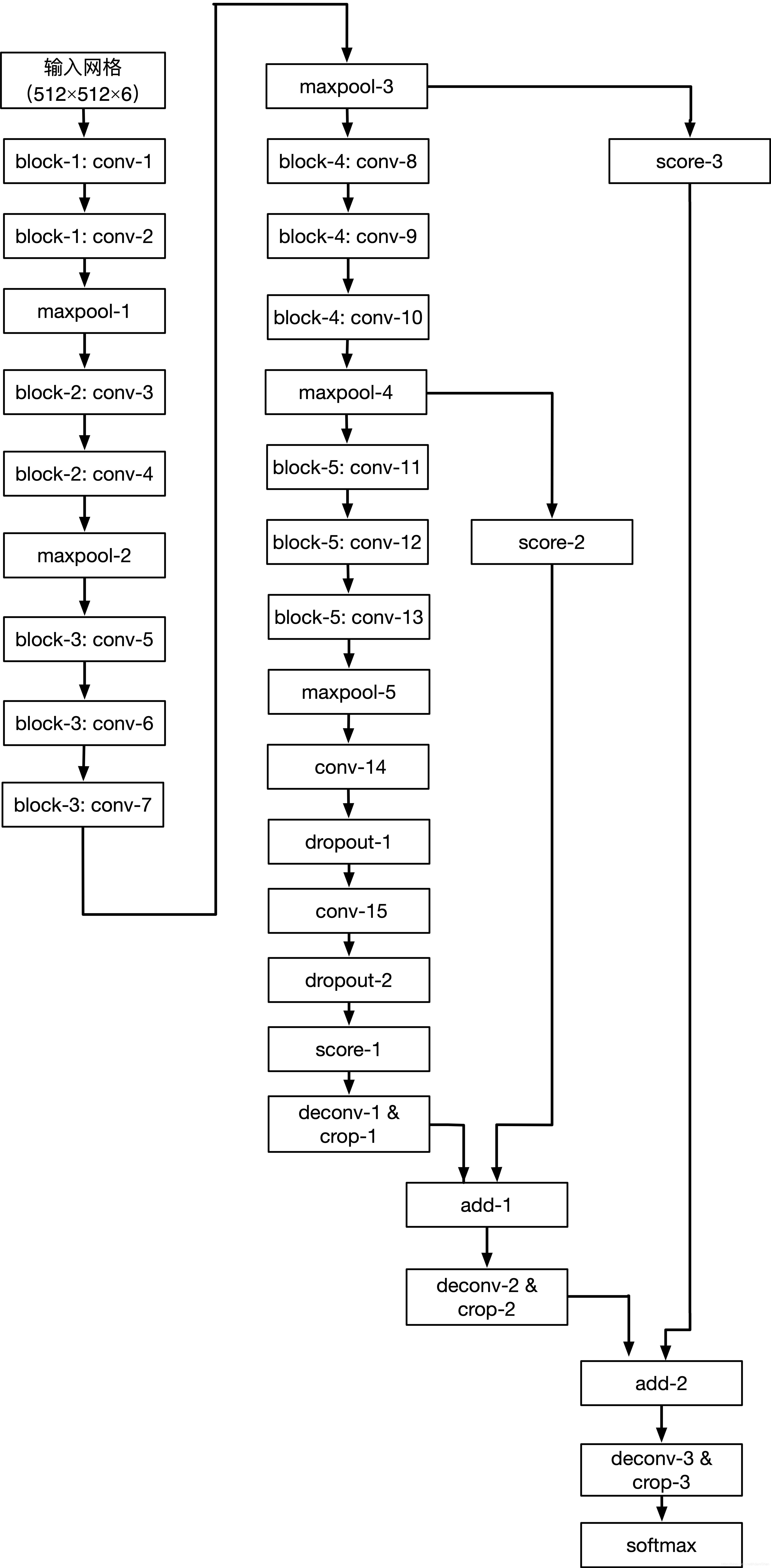
VGG16的结构大家应该比较熟悉，在此不赘述，由于解码器存在两个分支（分割分支和嵌入分支），所以该项目实现对FCN-VGG16的网络也做了调整，原来的编码器的block-5（卷积块）被分成两个分支，即从maxpool-4的输出分别被输入到两个卷积块，分别用于binary segment和instance segment。相对应的，两个编码输出到两个解码分支，对每一个卷积块的输出进行相应的上采样（使用反卷积上采样），并层层进行输出图逐元素叠加，可以得到两个分支分别输出的预测图（logits），这两部分logits被分别计算损失，使用交叉熵计算分割分支的损失 $L_{binary}$（带权重二分类，权重比为1.45:21.52）,使用上文所述的损失函数 $L_{instance} = L_{var} + L_{dist}$计算嵌入损失（用于同一车道线的像素聚类）。最后总的损失函数 $L_{total}$ 为：

$L_{total} = \frac{1}{2}L_{binary} + \frac{1}{2}L_{instance} + 0.001 \times L_{reg}$

其中 $L_{reg}$ 是参数的正则化。

训练

下载VGG16网络的预训练权重vgg16.npy，下载地址，下载完成以后将vgg16.npy 放到data目录下，然后使用脚本tools/train_lanenet.py 开始训练：

python tools/train_lanenet.py --dataset_dir ./data/training_data_example --multi_gpus False --net_flag vgg

使用tensorboard查看训练过程：

cd tboard/tusimple_lanenet_vgg/
tensorboard --logdir=.

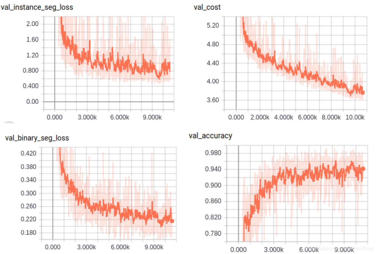
在训练过程中，可以通过tensorboard查看模型在验证集上的总损失(val_cost)、分割损失（val_binary_seg_loss）、嵌入损失（val_instance_seg_loss）以及分割精度（val_accuracy）变化曲线，如下所示：

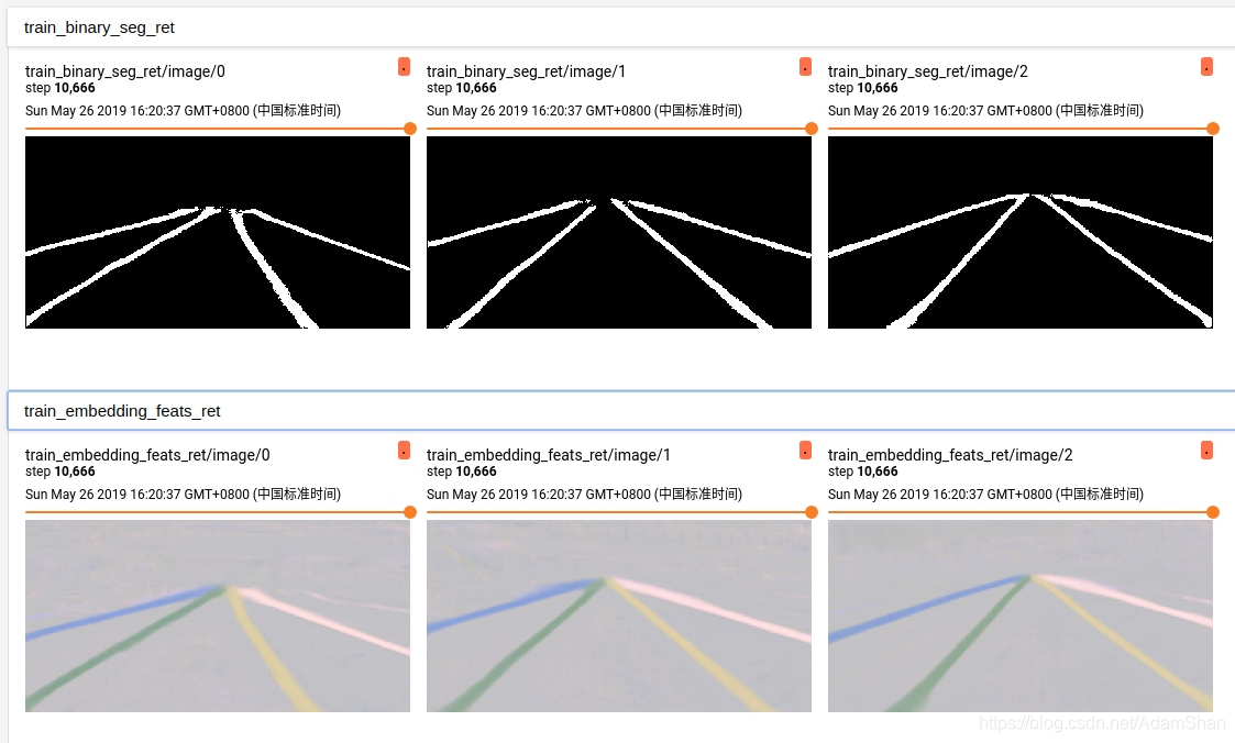
我们还可以查看模型在训练过程中的分割分支和嵌入分支输出到预测图，如下图所示：

模型在单个GPU上训练时间比较长，在我的主机（i7-8700, GTX1070）上，训练batch个epoch大约用时30个小时。

ROS节点

下面，我们修改lanenet-lane-detection项目为一个ROS节点，并且使用我们自己的数据（rosbag）验证训练的模型的车道线检测（本质上是分割）的效果。

项目地址：LaneNetRos

创建一个ROS的项目，下载预训练的LaneNet模型LaneNet，当然也可以直接使用按照上述步骤得出的我们自己训练的模型，将所有checkpoint文件拷贝至项目的 model/new_model/目录下。

我们看一下Ros节点script/lanenet_node.py代码：

import time
import math
import tensorflow as tf
import numpy as np
import cv2

from lanenet_model import lanenet
from lanenet_model import lanenet_postprocess
from config import global_config

import rospy
from sensor_msgs.msg import Image
from std_msgs.msg import Header
from cv_bridge import CvBridge, CvBridgeError
from lane_detector.msg import Lane_Image


CFG = global_config.cfg


class lanenet_detector():
    def __init__(self):
        self.image_topic = rospy.get_param('~image_topic')
        self.output_image = rospy.get_param('~output_image')
        self.output_lane = rospy.get_param('~output_lane')
        self.weight_path = rospy.get_param('~weight_path')
        self.use_gpu = rospy.get_param('~use_gpu')
        self.lane_image_topic = rospy.get_param('~lane_image_topic')

        self.init_lanenet()
        self.bridge = CvBridge()
        sub_image = rospy.Subscriber(self.image_topic, Image, self.img_callback, queue_size=1)
        self.pub_image = rospy.Publisher(self.output_image, Image, queue_size=1)
        self.pub_laneimage = rospy.Publisher(self.lane_image_topic, Lane_Image, queue_size=1)

    
    def init_lanenet(self):
        '''
        initlize the tensorflow model
        '''

        self.input_tensor = tf.placeholder(dtype=tf.float32, shape=[1, 256, 512, 3], name='input_tensor')
        phase_tensor = tf.constant('test', tf.string)
        net = lanenet.LaneNet(phase=phase_tensor, net_flag='vgg')
        self.binary_seg_ret, self.instance_seg_ret = net.inference(input_tensor=self.input_tensor, name='lanenet_model')

        # self.cluster = lanenet_cluster.LaneNetCluster()
        self.postprocessor = lanenet_postprocess.LaneNetPostProcessor()

        saver = tf.train.Saver()
        # Set sess configuration
        if self.use_gpu:
            sess_config = tf.ConfigProto(device_count={'GPU': 1})
        else:
            sess_config = tf.ConfigProto(device_count={'CPU': 0})
        sess_config.gpu_options.per_process_gpu_memory_fraction = CFG.TEST.GPU_MEMORY_FRACTION
        sess_config.gpu_options.allow_growth = CFG.TRAIN.TF_ALLOW_GROWTH
        sess_config.gpu_options.allocator_type = 'BFC'

        self.sess = tf.Session(config=sess_config)
        saver.restore(sess=self.sess, save_path=self.weight_path)

    
    def img_callback(self, data):
        try:
            cv_image = self.bridge.imgmsg_to_cv2(data, "bgr8")
        except CvBridgeError as e:
            print(e)
        original_img = cv_image.copy()
        resized_image = self.preprocessing(cv_image)
        mask_image = self.inference_net(resized_image, original_img)
        out_img_msg = self.bridge.cv2_to_imgmsg(mask_image, "bgr8")
        self.pub_image.publish(out_img_msg)
        
    def preprocessing(self, img):
        image = cv2.resize(img, (512, 256), interpolation=cv2.INTER_LINEAR)
        image = image / 127.5 - 1.0
        return image

    def inference_net(self, img, original_img):
        binary_seg_image, instance_seg_image = self.sess.run([self.binary_seg_ret, self.instance_seg_ret],
                                                        feed_dict={self.input_tensor: [img]})

        postprocess_result = self.postprocessor.postprocess(
            binary_seg_result=binary_seg_image[0],
            instance_seg_result=instance_seg_image[0],
            source_image=original_img
        )
        # mask_image = postprocess_result['mask_image']
        mask_image = postprocess_result
        mask_image = cv2.resize(mask_image, (original_img.shape[1],
                                                original_img.shape[0]),interpolation=cv2.INTER_LINEAR)
        mask_image = cv2.addWeighted(original_img, 0.6, mask_image, 5.0, 0)
        return mask_image


    def minmax_scale(self, input_arr):
        """

        :param input_arr:
        :return:
        """
        min_val = np.min(input_arr)
        max_val = np.max(input_arr)

        output_arr = (input_arr - min_val) * 255.0 / (max_val - min_val)

        return output_arr



if __name__ == '__main__':
    # init args
    rospy.init_node('lanenet_node')
    lanenet_detector()
    rospy.spin()

节点加载路径参数weight_path中的预训练的LaneNet模型权重，初始化整个网络，节点监听参数 image_topic 定义的话题，解析图像，并对图像进行预预处理（包括resize和归一化至-1.0～1.0）。最终的车道线分割结果被输出到由参数 output_image 定义的话题上。

接着是launch文件的编写：

<launch>

    <arg name="image_topic" default="/kitti/camera_color_left/image_raw"/>
    <arg name="output_image" default="/lane_images"/>
    <arg name="output_lane" default="/Lane"/>
    <arg name="weight_path" default="$(find lane_detector)/model/new_model/tusimple_lanenet.ckpt"/>

    <arg name="use_gpu" default="1"/>
    <arg name="lane_image_topic" default="/lane_image"/>

    <node pkg="lane_detector" type="lanenet_node.py" name="lanenet_node" output="screen">
        <param name="image_topic" value="$(arg image_topic)" />
        <param name="output_image" value="$(arg output_image)" />
        <param name="output_lane" value="$(arg output_lane)" />
        <param name="weight_path" value="$(arg weight_path)" />
        <param name="use_gpu" value="$(arg use_gpu)" />
        <param name="lane_image_topic" value="$(arg lane_image_topic)" />
    </node>
</launch>

我们使用kitti数据集制作一个rosbag用于测试,当然你也可以自己使用摄像头录制一段车道线的rosbag，下载任意一个包含车道线的原始的kitti数据片段：下载地址，注意只需要下载 synced+rectified data 和 calibration 文件。

使用kitti2bag 项目将原始数据转换成rosbag，使用说明见kitti2bag的github README。运行对于的kitti bag：

rosbag play kitti_2011_??????????.bag

打开rqt，使用Plugins->image viewer查看对应的原始图像和检测后的图像，如下图：

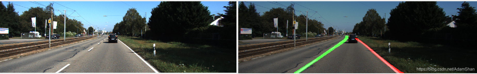
就lanenet-lane-detection项目而言，单纯使用tuSimple数据集训练的模型在kitti上的表现很一般，这和摄像头的分辨率等因素有关，读者可以自行构建数据集，以提升检测精度。

TODO

• LaneNetRos的曲线拟合（二次多项式拟合），主要是鸟瞰变换的remap关系如何简单计算
• 模型泛化能力有待提升
• 模型inference速度优化
• TensorRT优化