1. dplyr简介
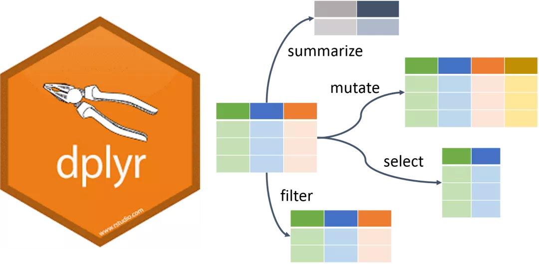
dplyr是R语言的数据分析包，类似于python中的pandas，能对dataframe类型的数据做很方便的数据处理和分析操作。最初我也很奇怪dplyr这个奇怪的名字，我查到其中一种解释 - d代表dataframe - plyr是英文钳子plier的谐音

dplyr如同R的大多数包，都是函数式编程，这点跟Python面向对象编程区别很大。优点是初学者比较容易接受这种函数式思维，有点类似于流水线，每个函数就是一个车间，多个车间共同完成一个生产（数据分析）任务。

而在dplyr中，就有一个管道符 %>% ，符号左侧表示数据的输入，右侧表示下游数据处理环节。

2. 安装并导入dplyr库
pacman库的p_load函数功能包含了

1. install.packages(“dplyr”)
2. library(dplyr)
   该写法更简单易用

pacman::p_load("dplyr")

**3. 读取数据**

#设置工作目录
setwd("/Users/thunderhit/Desktop/dplyr_learn")

#导入csv数据
aapl <- read.csv('aapl.csv',
header=TRUE,
sep=',',
stringsAsFactors = FALSE) %>% as_tibble()
head(aapl)

A tibble: 6 × 6
![](https://s4.51cto.com/images/blog/202012/30/e8ec6453c58ef833f05be96b520b3f66.png?x-oss-process=image/watermark,size_16,text_QDUxQ1RP5Y2a5a6i,color_FFFFFF,t_100,g_se,x_10,y_10,shadow_90,type_ZmFuZ3poZW5naGVpdGk=)
查看数据类型

class(aapl)

'tbl_df'

'tbl'

'data.frame'

查看数据的字段

colnames(aapl)

'Date'

'Open'

'High'

'Low'

'Close'

'Volume'

查看记录数、字段数

dim(aapl)

251

6

**4. dplyr常用函数**
**4.1 Arrange**
对appl数据按照字段Volume进行降序排序

arrange(aapl, -Volume)

A tibble: 6 × 6
![](https://s4.51cto.com/images/blog/202012/30/b85165f87b036f85be4f04d0b9440d7f.png?x-oss-process=image/watermark,size_16,text_QDUxQ1RP5Y2a5a6i,color_FFFFFF,t_100,g_se,x_10,y_10,shadow_90,type_ZmFuZ3poZW5naGVpdGk=)
我们也可以用管道符 %>% ，两种写法得到的运行结果是一致的，可能用久了会觉得管道符 %>% 可读性更强，后面我们都会用 %>% 来写代码。

aapl %>% arrange(-Volume)

A tibble: 6 × 6
![](https://s4.51cto.com/images/blog/202012/30/3bd99180a44d5679af4f84db43b961cd.png?x-oss-process=image/watermark,size_16,text_QDUxQ1RP5Y2a5a6i,color_FFFFFF,t_100,g_se,x_10,y_10,shadow_90,type_ZmFuZ3poZW5naGVpdGk=)
**4.2 Select**
选取 Date、Close和Volume三列

aapl %>% select(Date, Close, Volume)

![](https://s4.51cto.com/images/blog/202012/30/e8a9d430742058ef02e7d40c63ab0f76.png?x-oss-process=image/watermark,size_16,text_QDUxQ1RP5Y2a5a6i,color_FFFFFF,t_100,g_se,x_10,y_10,shadow_90,type_ZmFuZ3poZW5naGVpdGk=)
只选取Date、Close和Volume三列，其实另外一种表达方式是“排除Open、High、Low，选择剩下的字段的数据”。

aapl %>% select(-c("Open", "High", "Low"))

![](https://s4.51cto.com/images/blog/202012/30/05de7bd25514a8ddab6357ca7322ef7c.png?x-oss-process=image/watermark,size_16,text_QDUxQ1RP5Y2a5a6i,color_FFFFFF,t_100,g_se,x_10,y_10,shadow_90,type_ZmFuZ3poZW5naGVpdGk=)
**4.3 Filter**
按照筛选条件选择数据

#从数据中选择appl股价大于150美元的交易数据
aapl %>% filter(Close>=150)

![](https://s4.51cto.com/images/blog/202012/30/35242c4f0e45d7329e7033c0f64ef322.png?x-oss-process=image/watermark,size_16,text_QDUxQ1RP5Y2a5a6i,color_FFFFFF,t_100,g_se,x_10,y_10,shadow_90,type_ZmFuZ3poZW5naGVpdGk=)
从数据中选择appl - 股价大于150美元 且 收盘价大于开盘价 的交易数据

aapl %>% filter((Close>=150) & (Close>Open))

![](https://s4.51cto.com/images/blog/202012/30/2a75e95cf0cceed0d7fdee04930053bd.png?x-oss-process=image/watermark,size_16,text_QDUxQ1RP5Y2a5a6i,color_FFFFFF,t_100,g_se,x_10,y_10,shadow_90,type_ZmFuZ3poZW5naGVpdGk=)
**4.4 Mutate**
将现有的字段经过计算后生成新字段。

#将最好价High减去最低价Low的结果定义为maxDif，并取log
aapl %>% mutate(maxDif = High-Low,
log_maxDif=log(maxDif))

![](https://s4.51cto.com/images/blog/202012/30/1383ab8f2704ff082184be58e9a8cd09.png?x-oss-process=image/watermark,size_16,text_QDUxQ1RP5Y2a5a6i,color_FFFFFF,t_100,g_se,x_10,y_10,shadow_90,type_ZmFuZ3poZW5naGVpdGk=)
得到记录的位置(行数)

aapl %>% mutate(n=row_number())

![](https://s4.51cto.com/images/blog/202012/30/a6c2415852c4c7d5111adfb062909406.png?x-oss-process=image/watermark,size_16,text_QDUxQ1RP5Y2a5a6i,color_FFFFFF,t_100,g_se,x_10,y_10,shadow_90,type_ZmFuZ3poZW5naGVpdGk=)
**4.5 Group_By**
对资料进行分组，这里导入新的 数据集 weather

#导入csv数据
weather <- read.csv('weather.csv',
header=TRUE,
sep=',',
stringsAsFactors = FALSE) %>% as_tibble()
weather

![](https://s4.51cto.com/images/blog/202012/30/e67eb1810297ed7cc07633bcf4a01f49.png?x-oss-process=image/watermark,size_16,text_QDUxQ1RP5Y2a5a6i,color_FFFFFF,t_100,g_se,x_10,y_10,shadow_90,type_ZmFuZ3poZW5naGVpdGk=)
按照城市分组

weather %>% group_by(city)

![](https://s4.51cto.com/images/blog/202012/30/d6f71e09428e5262c64f7f9bcab295be.png?x-oss-process=image/watermark,size_16,text_QDUxQ1RP5Y2a5a6i,color_FFFFFF,t_100,g_se,x_10,y_10,shadow_90,type_ZmFuZ3poZW5naGVpdGk=)

为了让大家看到分组的功效，咱们按照城市分别计算平均温度

weather %>% group_by(city) %>% summarise(mean_temperature = mean(temperature))

`summarise()` ungrouping output (override with `.groups` argument)
![](https://s4.51cto.com/images/blog/202012/30/93a8b1d75bd558a4bd70515761c2bbd9.png?x-oss-process=image/watermark,size_16,text_QDUxQ1RP5Y2a5a6i,color_FFFFFF,t_100,g_se,x_10,y_10,shadow_90,type_ZmFuZ3poZW5naGVpdGk=)

weather %>% summarise(mean_temperature = mean(temperature))

![](https://s4.51cto.com/images/blog/202012/30/8e9afc255c68f598d06a104355e145f5.png?x-oss-process=image/watermark,size_16,text_QDUxQ1RP5Y2a5a6i,color_FFFFFF,t_100,g_se,x_10,y_10,shadow_90,type_ZmFuZ3poZW5naGVpdGk=)