衍生算法大合集

前言

这学期上计算智能课，感觉收获蛮多，然后实现了些书中的代码，以这篇博客来记录一下

• 神经网络
• 遗传算法
• 蚁群优化算法
• 粒子群算法
• 爬山法
• 模拟退火算法

本文链接: https://blog.csdn.net/weixin_43850253/article/details/109684307
这篇文章提到的课本如果没有特别说明，就是《计算智能》 张军 詹志辉等 编著， 清华大学出版社 2009年11月版 ，可能有同学觉得这本课本很老并且这篇博客算法简单，确实，这篇博客本身就是面向入门读者的。

神经网络

已知一个前馈型神经网络例子如下图所示. 设学习率 l (L的小写) 为0.9， 当前的训练样本为 x = {1,0,1}, 而且预期分类标号为1，同时，表2.3给出了当前该网络的各个连接权重和神经元偏置。求该网络在当前训练样本下的训练过程。

import math
import matplotlib.pyplot as plt


def network_2_1(x, t_6, l_r, precision=4, precision2=3):
    """
    模拟《计算智能》张军P15 2.1 的网络的代码
    :param x: x是一个三个元素的列表, 如[1, 0, 1]
    :param t_6: 六号神经元预期输出
    :param l_r: 学习率
    :param precision: 小数点后保留位数
    :param precision2: 小数点后保留位数
    :return: 参数和偏置
    """
    # 初始化网络的参数权重
    # 分别是 w_1_4, w_1_5, w_2_4, w_2_5, w_3_4, w_3_5, w_4_6, w_5_6
    w = [0.2, -0.3, 0.4, 0.1, -0.5, 0.2, -0.3, -0.2]
    # 分别是 xi_ta_4, xi_ta_5, xi_ta_6
    xi_ta = [-0.4, 0.2, 0.1]

    # 不断迭代并更新权重
    # 计算输出
    s_4 = w[0] * x[0] + w[2] * x[1] + w[4] * x[2] + xi_ta[0]
    o_4 = 1 / (1 + math.pow(math.e, -s_4))
    s_5 = w[1] * x[0] + w[3] * x[1] + w[5] * x[2] + xi_ta[1]
    o_5 = 1 / (1 + math.pow(math.e, -s_5))
    s_6 = w[6] * o_4 + w[7] * o_5 + xi_ta[2]
    o_6 = 1 / (1 + math.pow(math.e, -s_6))

    # 误差计算
    j_6 = o_6 * (1 - o_6) * (t_6 - o_6)
    j_5 = o_5 * (1 - o_5) * j_6 * w[7]
    j_4 = o_4 * (1 - o_4) * j_6 * w[6]

    # 神经元参数更新
    w[6] = w[6] + l_r * j_6 * o_4
    w[7] = w[7] + l_r * j_6 * o_5
    w[0] = w[0] + l_r * j_4 * x[0]
    w[1] = w[1] + l_r * j_5 * x[0]
    w[2] = w[2] + l_r * j_4 * x[1]
    w[3] = w[3] + l_r * j_5 * x[1]
    w[4] = w[4] + l_r * j_4 * x[2]
    w[5] = w[5] + l_r * j_5 * x[2]

    xi_ta[2] = xi_ta[2] + l_r * j_6
    xi_ta[1] = xi_ta[1] + l_r * j_5
    xi_ta[0] = xi_ta[0] + l_r * j_4

    # 输出一下
    print('每个神经元的总输入和输出计算表'.center(50, '-'))
    print('{:5} {:10} {:10}'.format(4, round(s_4, precision), round(o_4, precision2)))
    print('{:5} {:10} {:10}'.format(5, round(s_5, precision), round(o_5, precision2)))
    print('{:5} {:10} {:10}'.format(6, round(s_6, precision), round(o_6, precision2)))

    print()
    print('每个神经元的误差计算表'.center(50, '-'))
    print('{:5} {:10}'.format(6, round(j_6, precision)))
    print('{:5} {:10}'.format(5, round(j_5, precision)))
    print('{:5} {:10}'.format(4, round(j_4, precision)))

    print()
    print('网络连接权重和神经元偏置更新计算表'.center(50, '-'))
    print('{:10} {:10}'.format('w_4_6', round(w[6], precision2)))
    print('{:10} {:10}'.format('w_5_6', round(w[7], precision2)))
    print('{:10} {:10}'.format('w_1_4', round(w[0], precision2)))
    print('{:10} {:10}'.format('w_1_5', round(w[1], precision2)))
    print('{:10} {:10}'.format('w_2_4', round(w[2], precision2)))
    print('{:10} {:10}'.format('w_2_5', round(w[3], precision2)))
    print('{:10} {:10}'.format('w_3_4', round(w[4], precision2)))
    print('{:10} {:10}'.format('w_3_5', round(w[5], precision2)))
    print('{:10} {:10}'.format('xi_ta_6', round(xi_ta[2], precision2)))
    print('{:10} {:10}'.format('xi_ta_5', round(xi_ta[1], precision2)))
    print('{:10} {:10}'.format('xi_ta_4', round(xi_ta[0], precision2)))
    return w, xi_ta


def network_2_1_homework(x, t_6, l_r, accept_loss, iteration_max, precision=4, precision2=3):
    """
    模拟《计算智能》张军P15 2.1 的网络的代码,并将loss迭代到小于accept_loss
    :param x: x是一个三个元素的列表, 如[1, 0, 1]
    :param t_6: 六号神经元预期输出
    :param accept_loss:接受的误差
    :param l_r: 学习率
    :param iteration_max: 最大迭代次数
    :param precision: 小数点后保留位数
    :param precision2: 小数点后保留位数
    :return: 参数和偏置
    """
    # 初始化网络的参数权重
    # 分别是 w_1_4, w_1_5, w_2_4, w_2_5, w_3_4, w_3_5, w_4_6, w_5_6
    w = [0.2, -0.3, 0.4, 0.1, -0.5, 0.2, -0.3, -0.2]
    # 分别是 xi_ta_4, xi_ta_5, xi_ta_6
    xi_ta = [-0.4, 0.2, 0.1]
    loss = accept_loss + 5

    # 不断迭代并更新权重
    run_times = 0  # 迭代次数
    loss_lt = []  # 误差数组

    generation = 0
    while loss > accept_loss and generation < iteration_max:
        generation += 1
        # 计算输出
        s_4 = w[0] * x[0] + w[2] * x[1] + w[4] * x[2] + xi_ta[0]
        o_4 = 1 / (1 + math.pow(math.e, -s_4))
        s_5 = w[1] * x[0] + w[3] * x[1] + w[5] * x[2] + xi_ta[1]
        o_5 = 1 / (1 + math.pow(math.e, -s_5))
        s_6 = w[6] * o_4 + w[7] * o_5 + xi_ta[2]
        o_6 = 1 / (1 + math.pow(math.e, -s_6))

        # 误差计算
        j_6 = o_6 * (1 - o_6) * (t_6 - o_6)
        j_5 = o_5 * (1 - o_5) * j_6 * w[7]
        j_4 = o_4 * (1 - o_4) * j_6 * w[6]

        # 神经元参数更新
        w[6] = w[6] + l_r * j_6 * o_4
        w[7] = w[7] + l_r * j_6 * o_5
        w[0] = w[0] + l_r * j_4 * x[0]
        w[1] = w[1] + l_r * j_5 * x[0]
        w[2] = w[2] + l_r * j_4 * x[1]
        w[3] = w[3] + l_r * j_5 * x[1]
        w[4] = w[4] + l_r * j_4 * x[2]
        w[5] = w[5] + l_r * j_5 * x[2]

        xi_ta[2] = xi_ta[2] + l_r * j_6
        xi_ta[1] = xi_ta[1] + l_r * j_5
        xi_ta[0] = xi_ta[0] + l_r * j_4

        loss = t_6 - o_6
        loss_lt.append(loss)
        run_times += 1  # 迭代次数加一

    print('迭代次数 {}， 最终误差 {}'.format(run_times, loss_lt[-1]))
    print('网络连接权重和神经元偏置更新计算表'.center(50, '-'))
    print('{:10} {:10}'.format('w_4_6', round(w[6], precision2)))
    print('{:10} {:10}'.format('w_5_6', round(w[7], precision2)))
    print('{:10} {:10}'.format('w_1_4', round(w[0], precision2)))
    print('{:10} {:10}'.format('w_1_5', round(w[1], precision2)))
    print('{:10} {:10}'.format('w_2_4', round(w[2], precision2)))
    print('{:10} {:10}'.format('w_2_5', round(w[3], precision2)))
    print('{:10} {:10}'.format('w_3_4', round(w[4], precision2)))
    print('{:10} {:10}'.format('w_3_5', round(w[5], precision2)))
    print('{:10} {:10}'.format('xi_ta_6', round(xi_ta[2], precision2)))
    print('{:10} {:10}'.format('xi_ta_5', round(xi_ta[1], precision2)))
    print('{:10} {:10}'.format('xi_ta_4', round(xi_ta[0], precision2)))
    return w, xi_ta, loss_lt


def draw(loss_lt, string):
    """
    绘图出损失凸显
    :param loss_lt: 损失值的列表
    :param string: 图标的标题
    :return: none
    """
    # 第二个图
    x = list(range(len(loss_lt)))
    y = loss_lt
    plt.xlim(0, len(loss_lt) + 1)
    # 为了显示中文，指定默认字体
    plt.rcParams['font.sans-serif'] = ['SimHei']
    plt.plot(x, y, 'b-')
    plt.title(string, fontsize=22, fontweight='light', color='w', backgroundcolor='g')
    plt.show()


if __name__ == '__main__':
    # network_2_1([1, 0, 1], 1, 0.9)
    _, _, loss_list = network_2_1_homework([1, 0, 1], 1, 0.9, 0.1, 100)
    draw(loss_list, '误差变化图')

其中 network_2_1只是为了验证模型是否与书中的算出来一样，大家可以忽略。
运行结果:

遗传算法

已知函数
$$y=f(x_1,x_2,x_3,x_4)=\frac{1}{x_1^2+x_2^2+x_3^2+x_4^2}$$
其中，-5 ≤ x₁, x₂, x₃, x₄, 用遗传算法求解y的最大值。

"""
课本第64页例题遗传算法
"""
"""
@author: Andy Dennis
@time: 2020/10/24
@detail: 感悟，拷贝二维数组一定要深拷贝，不然找bug有你好玩的! 别偷懒，建议双重循环拷贝...
"""
# %%
import random


def genetic(value_range, fitness_func, N, c_l, Pc, Pm, G_max, accept_value):
    """
    遗传算法
    :param value_range: 取值范围 [min, max]
    :param fitness_func: 适应度函数的字符串
    :param c_l: 染色体长度
    :param N: 种群规模
    :param Pc: 交配概率
    :param Pm: 变异概率
    :param G_max: 最大进化代数
    :param accept_value: 可接受的解,包含这个数值
    :return: 一组较优解和对应的最大值
    """
    # 步骤一, 初始化
    group = []
    for i in range(N):
        # random.random()  [min, max]
        group.append([random.uniform(value_range[0], value_range[1]) for j in range(c_l)])
    # print_group(group, ' initial group ')
    # print()

    # 步骤二，适应值评价
    eval_lt = []
    for i in group:
        eval_lt.append(eval(fitness_func)(i))
    # print('eval_lt: ', eval_lt)
    best_result = max(eval_lt)
    best_solution = [group[i] for i in range(len(group)) if eval_lt[i] == best_result][0]
    # print('初始best_result: ', best_result)
    # print('{} -> {}'.format(best_solution, best_result))
    # print()

    generation_num = 0
    while best_result < accept_value and generation_num < G_max:
        generation_num += 1
        # 步骤三，选择
        sum_eval = sum(eval_lt)
        share_lt = [i / sum_eval for i in eval_lt]
        for i in range(1, len(share_lt)):
            share_lt[i] += share_lt[i - 1]

        choose_lt = []
        for i in range(N):
            random_num = random.random()
            for j in range(len(share_lt)):
                if random_num <= share_lt[j]:
                    choose_lt.append(j)
                    break
        # print('选中交配的个体: ', choose_lt)
        temp = group[:]
        group.clear()
        # 注意要深拷贝，不然会导致交配那部分产生逻辑错误
        group = [[j for j in temp[i]] for i in choose_lt]
        # print_group(group, ' 选中后的个体 ')
        # print()

        # 步骤四，交配
        mating_lt = []
        is_ok = False
        while not is_ok:
            mating_lt.clear()
            for i in range(len(choose_lt)):
                if random.random() <= Pc:
                    mating_lt.append(i)
            if len(mating_lt) % 2 == 0:
                is_ok = True

        # print('mate_lt: ', mating_lt)

        leave_group, mate_group = [], []
        leave_group.clear()
        mate_group.clear()
        for i in range(N):
            if i in mating_lt:
                mate_group.append(group[i])
            else:
                leave_group.append(group[i])
        # leave_group = [group[i] for i in range(N) if i not in mating_lt]
        # mate_group = [group[i] for i in range(N) if i in mating_lt]
        # print_group(leave_group, ' 保持原样的种群 leave_group ')
        # print_group(mate_group, ' 进行交配的种群 mate_group ')
        group.clear()

        # 开始两两交配
        mate_i = 0
        while mate_i < len(mating_lt):
            position = random.randrange(c_l - 1)
            # print('position: ', position)
            mate_group[mate_i][position + 1:], mate_group[mate_i + 1][position + 1:] = \
                mate_group[mate_i + 1][position + 1:], mate_group[mate_i][position + 1:]
            # print('mate_i: ', mate_i, mating_lt)
            # print_group(leave_group, ' log leave_group ')
            mate_i += 2
        for i in leave_group:
            group.append(i)
        for i in mate_group:
            group.append(i)
        # print_group(leave_group, ' 遗留的种群 leave_group ')
        # print_group(mate_group, ' 交配done的种群 mate_group ')
        # print_group(group, ' 交配后的种群 group ')
        # print()

        # 第五步，变异
        for i in range(len(group)):
            for j in range(c_l):
                if random.random() <= Pm:
                    group[i][j] = random.uniform(value_range[0], value_range[1])
        # print_group(group, ' 变异后的group ')
        # print()

        # 步骤六, 重新评价染色体适应值，更新besgt
        eval_lt = []
        for i in group:
            eval_lt.append(eval(fitness_func)(i))
        # print('eval_lt: ', eval_lt)
        if max(eval_lt) > best_result:
            print('更新啦...')
            best_result = max(eval_lt)
            best_solution = [group[i] for i in range(len(group)) if eval_lt[i] == best_result][0]
            print('gen_{}: {} -> {}'.format(generation_num, best_solution, best_result))
    print('\nfinal:\n best_solution{} \n best_value: {}'.format(best_solution, best_result))


def print_group(g, string):
    # 打印群体
    print(string.center(50, '*'))
    for i in g:
        print(i)


def fit(x_lt):
    return 1 / (x_lt[0] ** 2 + x_lt[1] ** 2 + x_lt[2] ** 2 + x_lt[3] ** 2 + 1)


if __name__ == '__main__':
    genetic([-5, 5], 'fit', 5, 4, 0.88, 0.1, 200, 0.5)

运行结果:

蚁群优化算法

用蚁群优化算法求解四城市的TSP问题的执行步骤，四个城市A、B、C、D之间的距离矩阵如下:
$$W=d_{ij}=\left[\begin{array}{cccc}inf& 3& 1& 2\\ 3& inf& 5& 4\\ 1& 5& inf& 2\\ 2& 4& 2& inf\end{array}\right]$$
假设蚂蚁种群的规模为m = 3, 参数 α = 1, β = 2, ρ = 0.5。

"""
@author: Andy Dennis
@time: 2020/11/6
@detail: 课本P87 例 5.1
"""
import sys
import random


def aco_travel(m, d, a, beta, rou, accept_solve, G):
    """
    一群算法
    :param m: 蚂蚁种群规模
    :param d: 距离矩阵
    :param a: 信息素次幂权重
    :param beta: 启发式次幂权重
    :param rou:蒸发量
    :param accept_solve: 可接受的解，即最小距离是多少的时候可以停止
    :param G: 最大循环代数
    :return:
    """
    global inf

    city_num = len(d)
    R_best = inf
    R_best_path = []
    # 初始化
    # 贪婪算法
    c, _ = find_greedy(d)
    # print(c, _)
    tau = m / c
    tau_matrix = [[tau for j in range(city_num)] for i in range(city_num)]
    # print('{}\n{}'.format("tau_matrix initial:", tau_matrix))

    for generation in range(G):
        print()
        print(' 第 {} 代蚂蚁 '.format(generation + 1).center(50, '*'))

        # 步骤2.1-2.4
        # 为每只蚂蚁选择城市
        ant_choose = [[random.randint(0, city_num - 1)] for i in range(m)]

        for k in range(city_num - 1):
            for i in range(m):  # m 只蚂蚁
                # 保存中间结果
                temp_lt = []
                for j in range(city_num):  # city_num 个城市
                    if j not in ant_choose[i]:  # 还没走过
                        temp_p = tau ** a * (1 / d[ant_choose[i][-1]][j]) ** beta
                        temp_lt.append([temp_p, j])
                temp_lt.sort(key=lambda i: -i[0])
                temp_total_p = sum([item[0] for item in temp_lt])
                temp_lt = [[item[0] / temp_total_p, item[1]] for item in temp_lt]

                # 轮盘赌
                for j in range(1, len(temp_lt)):
                    temp_lt[j][0] += temp_lt[j - 1][0]
                random_num = random.random()
                for j in range(len(temp_lt)):
                    if temp_lt[j][0] >= random_num:
                        # 选择此时的城市作为第 i 只蚂蚁的下一个城市, 注意此时的编号是 temp_index_lt 的编号
                        ant_choose[i].append(temp_lt[j][1])
                        break

        # 最后要回到起点
        for i in range(m):
            ant_choose[i].append(ant_choose[i][0])

        print('蚂蚁们的选择:')
        print_matrix(ant_choose)

        # 步骤 3, 信息素的更新
        # 计算每只蚂蚁走过的路劲长度
        # 这里要开一个 city_num * city_num 的三维度矩阵，初始值为空，这个列表代表走过的蚂蚁编号
        flag_matrix = [[[] for i in range(city_num)] for j in range(city_num)]
        # print('flag_matrix initial: ')
        # print(flag_matrix)

        for i in range(m):  # m只蚂蚁
            for j in range(city_num - 1):  # m个城市
                # print(ant_choose[i][j], ant_choose[i][j + 1])
                flag_matrix[ant_choose[i][j]][ant_choose[i][j + 1]].append(i)  # 这条路 i 号蚂蚁走过了
        # print(flag_matrix)

        # 计算一项每只蚂蚁走过的路径长度
        c_lt = []
        for i in range(m):
            c_lt.append(sum([d[ant_choose[i][j]][ant_choose[i][j + 1]] for j in range(city_num)]))

        min_path_c = min(c_lt)
        min_path_index = [index for index, value in enumerate(c_lt) if value == min_path_c]

        # 更新信息素
        for i in range(m):
            for j in range(m):
                tau_matrix[i][j] = (1 - rou) * tau_matrix[i][j]
                for k in range(len(flag_matrix[i][j])):
                    tau_matrix[i][j] += 1 / c_lt[flag_matrix[i][j][k]]

        print('信息素更新新:')
        print_matrix(tau_matrix)

        if min_path_c < R_best:
            R_best = min_path_c
            R_best_path = [ant_choose[i] for i in min_path_index]

        print('此时最优值: {}, 最优路径: {}'.format(R_best, R_best_path))

        # 判断是否可以结束
        if R_best <= accept_solve:
            break
    return R_best, R_best_path


def find_greedy(d):
    # 路径
    route_lt = [0]
    # 贪婪算法得出的最短的路径
    route_size = 0
    for i in range(len(d) - 1):
        min_path = inf
        min_index = 0
        for j in range(len(d[0])):
            if j not in route_lt and d[route_lt[-1]][j] < min_path:
                min_index = j
                min_path = d[route_lt[-1]][j]
        route_size += min_path
        route_lt.append(min_index)
    # 返回原点的路程
    route_size += d[route_lt[-1]][0]
    route_lt.append(0)
    return route_size, route_lt


def print_matrix(d, precision=2):
    for i in range(len(d)):
        for j in range(len(d[0])):
            print('{:8}'.format(round(d[i][j], precision)), end='')
        print()


if __name__ == '__main__':
    inf = sys.maxsize
    w = [[inf, 3, 1, 2],
         [3, inf, 5, 4],
         [1, 5, inf, 2],
         [2, 4, 2, inf]]
    best_solve, best_path = aco_travel(3, w, 1, 2, 0.5, 9.9, 100)

    print()
    print('全局最优解: ', best_solve)
    print('全局最优路径: ', best_path)

运行结果:(只截取了一部分)

思考: 这里想着好像很长时间其实都陷入在局部最优解，我觉得应该可以加入一个机制: 很长时间出于平滑的区间的话，其实可以提前结束。

粒子群算法

已知函数
$$y=(x_1,x_2)=x_1^2+x_2^2$$
其中， -10 ≤ x₁ , x₂ ≤ 10, 用粒子群优化算法求解 y 的最小值。

"""
@author Andy Dennis
@date 2020/11/13
@detail 课本P113 例题6.1
其中矩阵运算部分还是比较耗时一些，建议可以使用numpy进行矢量运算加快运算速度,
不过此题运算量小，迭代次数就算是10000次也很快
但是经过实验我发现这个算法得到解的情况很不稳定...
"""
import random


def pso(N: int, D: int, w: float, c: list, func: str, iteration_num: int, accept_value: float,
        x_range: list, v_range: list = None, syn: bool = True):
    """
    模拟粒子群算法
    :param N: 种群数量
    :param D: 觅食空间，解的维度
    :param w: 惯量权重
    :param c: 加速系数, [c1, c2]
    :param func: 适应度函数
    :param iteration_num: 最大迭代次数，建议500~1000
    :param accept_value: 可接受的解的值(包含这个数)
    :param x_range: 位置x取值范围 [min, max]
    :param v_range: 速度v取值范围 [min, max]
    :param syn: True: 同步更新, False: 异步更新
    :return: 最优的一组解和最优解的值
    """
    # 步骤一，初始化
    if v_range is not None:
        v_lt = [[random.randint(v_range[0], v_range[1]) for j in range(D)] for i in range(N)]
    else:  # 默认初始化的速度在 20% 的解空间里
        length_range = x_range[1] - x_range[0]
        v_lt = [[random.randint(x_range[0] + length_range * 2 / 5,
                                x_range[0] + length_range * 3 / 5) for j in range(D)]
                for i in range(N)]
    x_lt = [[random.randint(x_range[0], x_range[1]) for j in range(D)] for i in range(N)]

    # print('initial speed vector:')
    # for i in v_lt:
    #     print(i)
    # print('initial position vector:')
    # for i in x_lt:
    #     print(i)

    # 存放每一个例子的历史最优
    p_best_lt = [[j for j in i] for i in x_lt]
    g_best = [i for i in x_lt[0]]
    g_best_value = eval(func)(x_lt[0][0], x_lt[0][1])
    # 加入第一个例子的历史最优值
    p_best_value_lt = [g_best_value]
    # 找出现阶段全局最优解
    for i in range(1, N):
        temp = eval(func)(x_lt[i][0], x_lt[i][1])
        # 将其加入每一个例子的历史最优值
        p_best_value_lt.append(temp)
        if temp < g_best_value:
            g_best_value = temp
            g_best = [j for j in x_lt[i]]
    print('g_best: {}, g_best_value: {}'.format(g_best, g_best_value))
    print()

    generation_num = 0
    while generation_num < iteration_num and g_best_value > accept_value:
        generation_num += 1
        # 步骤2 例子的速度和位置跟新
        for i in range(N):
            for j in range(D):
                # 速度向量更新
                v_lt[i][j] = w * v_lt[i][j] + c[0] * random.random() * (p_best_lt[i][j] - x_lt[i][j])
                + c[1] * random.random() * (g_best[j] - x_lt[i][j])
                # 更新位置向量
                x_lt[i][j] = x_lt[i][j] + v_lt[i][j]
                # 对于越界要进行合法性调整
                if x_lt[i][j] < x_range[0]:
                    x_lt[i][j] = x_range[0]
                if x_lt[i][j] > x_range[1]:
                    x_lt[i][j] = x_range[1]

        # 步骤3 评估例子的适应度函数值
        for i in range(N):
            temp = eval(func)(x_lt[i][0], x_lt[i][1])
            if temp < p_best_value_lt[i]:
                p_best_lt[i] = [j for j in x_lt[i]]
                p_best_value_lt[i] = temp
                # 异步更新
                if not syn and temp < g_best_value:
                    g_best_value = temp
                    g_best = [j for j in x_lt[i]]
                    print('gen_num_{}更新啦...\n g_best: {}, g_best_value: {}'.format(generation_num, g_best, g_best_value))
        if syn:  # 同步更新
            for i in range(len(p_best_value_lt)):
                if p_best_value_lt[i] < g_best_value:
                    g_best_value = p_best_value_lt[i]
                    g_best = p_best_lt[i]
                    print('gen_num_{}更新啦...\n g_best: {}, g_best_value: {}'.format(generation_num, g_best, g_best_value))
        # print('updated speed vector:')
        # for i in v_lt:
        #     print(i)
        # print('updated position vector:')
        # for i in x_lt:
        #     print(i)
        # print('gen_num_{} g_best: {}, g_best_value: {}'.format(generation_num, g_best, g_best_value))
    print()
    print('final g_best: {}, g_best_value: {}'.format(g_best, g_best_value))
    return g_best, g_best_value


def fc(x1, x2):
    return x1 ** 2 + x2 ** 2


if __name__ == '__main__':
    pso(N=3, D=2, w=0.5, c=[2, 2], func='fc', iteration_num=1000,
        accept_value=0.1, x_range=[-10, 10])

运行结果:(截取部分)

思考: 这里用到的是全局更新的策略，收敛速度快但比较容易陷入局部最优解。还有这里pco函数有个参数syn，如果设置为false的话， 就是异步更新啦

爬山法

已知函数
$$y=(x_1,x_2)=x_1^2+x_2^2$$
其中， -10 ≤ x₁ , x₂ ≤ 10, 用粒子群优化算法求解 y 的最小值。

1. 最快上升爬山法

# %%
"""
最快上升爬山法
x0 <- 随机生成个体
while not (结束条件)
    计算x0适应度
    for 对于解的每一个特征 q = 1, 2, ..., n
        xq = x0
        用一个随机变量替换xq的第q个特征
        计算xq的适应度
        再算下一个解特征
    x_max = 虽有变异的xq的可能中找出适应度最好的x_best
    if x0 == x_max then
        x0 = 随机生成个体
    else
        x0 = x_max
    下一代
"""
import random


def fc(x1, x2):
    return x1 ** 2 + x2 ** 2


# %%
def fastest_rise(func: str):
    """
    依次上升爬山法
    :param func: 适应度函数
    :return: 最优解和最优解得出的结果
    """
    D = 2  # 解的维度
    x_min, x_max = -10, 10  # 解的范围
    max_iter = 1000  # 最大迭代次数

    x0 = [random.uniform(x_min, x_max) for i in range(D)]
    iteration_num = 0
    x_best = [item for item in x0]
    x_best_value = eval(func)(x0[0], x0[1])
    while iteration_num < max_iter:
        iteration_num += 1
        x_best = [item for item in x0]
        x_best_value = eval(func)(x0[0], x0[1])
        for i in range(D):
            x_q = [item for item in x0]
            x_q[i] = random.uniform(x_min, x_max)
            fitness = eval(func)(x_q[0], x_q[1])
            # 这里更小适应度更优
            if fitness < x_best_value:
                x_best = [item for item in x_q]
                x_best_value = fitness
        if x0 == x_best:
            x0 = [random.uniform(x_min, x_max) for i in range(D)]
        else:
            x0 = [item for item in x_best]
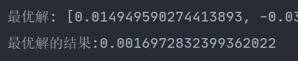
    print('最优解: {}\n最优解的结果:{}'.format(x_best, x_best_value))
    return x_best, x_best_value


fastest_rise('fc')

效果嘛，大家试试就知道了，可能迭代次数要加多一些。零点几的也有，几十也有，性能不稳定。

2. 依次上升爬山法

# %%
"""
依次上升爬山法 (最贪婪)
x0 <- 随机生成个体
while not (结束条件)
    计算x0适应度
    replaceFlag = false
    for 对于解的每一个特征 q = 1, 2, ..., n
        xq <- x0
        用一个随机变量替换xq的第q个特征
        计算xq的适应度
        if f(xq 适应度优于 x0)
            x0 = xq
            replaceFlag = true
    if not replaceFlag then
        x0 = 随机产生的个体
    下一代
"""
import random


def fc(x1, x2):
    return x1 ** 2 + x2 ** 2


# %%
def ascending(func: str):
    """
    依次上升爬山法
    :param func: 适应度函数
    :return: 最优解和最优解得出的结果
    """
    D = 2  # 解的维度
    x_min, x_max = -10, 10  # 解的范围
    max_iter = 1000  # 最大迭代次数

    x0 = [random.uniform(x_min, x_max) for i in range(D)]
    iteration_num = 0
    x0_fitness = eval(func)(x0[0], x0[1])
    while iteration_num < max_iter:
        iteration_num += 1
        x0_fitness = eval(func)(x0[0], x0[1])
        replaceFlag = False
        for i in range(D):
            x_q = [item for item in x0]
            x_q[i] = random.uniform(x_min, x_max)
            fitness = eval(func)(x_q[0], x_q[1])
            if fitness < x0_fitness:
                x0 = [item for item in x_q]
                replaceFlag = True
        if not replaceFlag:
            x0 = [random.uniform(x_min, x_max) for i in range(D)]
    x0_fitness = eval(func)(x0[0], x0[1])
    print('最优解: {}\n最优解的结果:{}'.format(x0, x0_fitness))
    return x0, x0_fitness


ascending('fc')

迭代1000次的性能比最快上升爬山法还要不稳定，可见贪婪不一定笑到最后。

3. 随机变异爬山法

# %%
"""
随机变异爬山法
x0 <- 随机生成个体
while not (结束条件)
    计算x0适应度
    q = 随机选择特征指标 [1, n]
    x1 = x0
    用一个随机变量替换x1的第q个特征
    计算x1的适应度
    if x1的适应度优于x0:
        x0 = x1
"""
import random


def fc(x1, x2):
    return x1 ** 2 + x2 ** 2


# %%
def random_variation(func: str):
    """
    随机变异爬山法
    :param func: 适应度函数
    :return: 最优解和最优解得出的结果
    """
    D = 2  # 解的维度
    x_min, x_max = -10, 10  # 解的范围
    max_iter = 1000  # 最大迭代次数

    x0 = [random.uniform(x_min, x_max) for i in range(D)]
    iteration_num = 0
    while iteration_num < max_iter:
        iteration_num += 1
        x0_fitness = eval(func)(x0[0], x0[1])
        x1 = [item for item in x0]
        x1[random.randint(0, D - 1)] = random.uniform(x_min, x_max)
        if eval(func)(x1[0], x1[1]) < x0_fitness:
            x0 = [item for item in x1]
    x0_fitness = eval(func)(x0[0], x0[1])
    print('最优解: {}\n最优解的结果:{}'.format(x0, x0_fitness))
    return x0, x0_fitness


random_variation('fc')

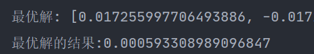
这性能没话说…和下面要讲到的自适应爬山法算是四种最好的吧(我们知道求原函数最小值是0)。

4. 自适应爬山法

# %%
"""
自适应爬山法
初始化 P_m 属于 [0, 1] 作为变异概率
x0 = 随机产生的个体
while not (终止条件):
    x1 = x0
    for 解的每一个特征 q = 1,2,...,n
        生成一个均匀随机数 r 属于 [0, 1]
        if r < p_m then
            用一个随机变量替换 x1 的第 q 个特征
    if x1 的适应度优于 x0
        x0 = x1
"""
import random


def fc(x1, x2):
    return x1 ** 2 + x2 ** 2


# %%
def adaptive_climbing(func: str):
    """
        随机变异爬山法
        :param func: 适应度函数
        :return: 最优解和最优解得出的结果
        """
    D = 2  # 解的维度
    x_min, x_max = -10, 10  # 解的范围
    max_iter = 1000  # 最大迭代次数

    p_m = random.random()
    x0 = [random.uniform(x_min, x_max) for i in range(D)]
    iteration_num = 0
    while iteration_num < max_iter:
        iteration_num += 1
        x1 = [item for item in x0]
        for i in range(D):
            r = random.random()
            if r < p_m:
                x1[i] = random.uniform(x_min, x_max)
        if eval(func)(x1[0], x1[1]) < eval(func)(x0[0], x0[1]):
            x0 = [item for item in x1]
    x0_fitness = eval(func)(x0[0], x0[1])
    print('最优解: {}\n最优解的结果:{}'.format(x0, x0_fitness))
    return x0, x0_fitness


adaptive_climbing('fc')

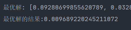
算是也比较好的。

5. 四种爬山法总结

最快上升爬山法和依次上升爬山法在小的迭代次数里容易陷入局部最优，性能不稳定。而随机变异和自适应算法由于解的变异情况多，跳出最优解的能力较强，效果会比前两者更好些。

模拟退火算法

已知函数
$$y=(x_1,x_2)=x_1^2+x_2^2$$
其中， -10 ≤ x₁ , x₂ ≤ 10, 用粒子群优化算法求解 y 的最小值。

# %%
"""
模拟退火算法
@Author: Andy Dennis
"""
import random
import math


def fc(x1, x2):
    return x1 ** 2 + x2 ** 2


# %%
def simulated_annealing(func: str):
    """
    模拟退火算法
    :param func: 适应度函数
    :return: 最优解和最优解得出的结果
    """
    D = 2  # 解的维度
    x_min, x_max = -10, 10  # 解的范围
    quick_flag = False  # True使用快速模拟退火降温标志(False则是使用经典退火算法的降温方式)
    max_iter = 1000  # 最大迭代次数, 当然这里也可以不用迭代次数而用温度来作为结束条件
    K = 1.380649 * 10 ** (-23)  # 玻尔兹曼常量
    # K = 1

    # 计算初始温度, 这一步也不是必须的，比如在这个问题下，
    # 我们取可能的适应度相差最大值最为初始温度就可以了, t = 200
    fitness_min, fitness_max = math.inf, -math.inf
    sample_num = 20  # 抽样个数
    x0 = [random.uniform(x_min, x_max) for i in range(D)]
    for i in range(sample_num):
        x_new = [item for item in x0]
        x0[random.randint(0, 1)] = random.uniform(x_min, x_max)
        fitness = eval(func)(x0[0], x0[1])
        if fitness < fitness_min:
            fitness_min = fitness
        if fitness > fitness_max:
            fitness_max = fitness
    # 初始温度就确定下来了，在这个问题中也可以直接取 200,
    # 这里我采用抽样的方法是因为有些问题不是很容易看出适应度相差大小
    t = fitness_max - fitness_min

    k = 0  # k代表迭代次数
    while k < max_iter and t > 10 ** (-5):
        k += 1
        fitness = eval(func)(x0[0], x0[1])
        for i in range(D):
            x_new = [item for item in x0]
            x_new[i] = random.uniform(x_min, x_max)
            fitness_new = eval(func)(x_new[0], x_new[1])
            if fitness_new < fitness:
                # 适应度更优, 直接转换
                x0 = [item for item in x_new]
            else:
                random_num = random.random()
                # 接受适应度不好的概率，此步骤在于保证解的多样性，增加避免陷入局部最优解的能力
                change_probability = math.exp(-(fitness_new - fitness) / (K * t))
                if random_num <= change_probability:
                    x0 = [item for item in x_new]
        if quick_flag:  # 快速降温
            t = t / (1 + k)
        else:  # 经典降温
            t = t / math.log(1 + k)

    x0_fitness = eval(func)(x0[0], x0[1])
    print('经过 {} 代后的最优解: {}\n最优解的结果:{}'.format(k, x0, x0_fitness))
    return x0, x0_fitness


simulated_annealing('fc')

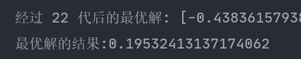
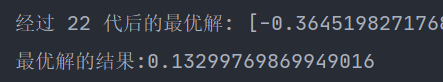
可以看到模拟退火算法虽然只迭代了22次，但是效果还是很可以的。这里状态的改变我是从用了变异的形式(下面一句代码)，读者也可以考虑其他状态改变。

x_new[i] = random.uniform(x_min, x_max)

结语

这些仿生学算法是我们计算机领域模拟动物界一些策略产生的优化问题的解决方案。在一些调度和优化问题上有广泛的应用。本文例子可能有些同学会觉得，这不是一眼就能看出结果的吗，为何还要用程序来算。其实这只是举个简单的例子，帮助理解，实际解决的问题很少有这么简单的(适应度函数那里)。