AlexNet
AlexNet网络的优点:
- 首次利用GPU进行网络加速训练
- 使用了ReLU激活函数,而不是传统的Sigmoid激活函数以及Tanh激活函数
- 使用了LRN局部响应归一化
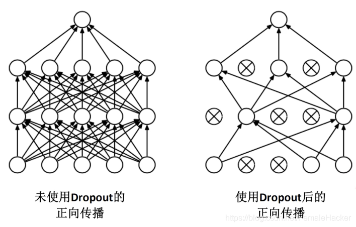
- 在全连接层的前两层中使用了Dropout随机失活神经元操作,以减少过拟合。
过拟合:根本原因是特征维度过多,模型假设过于复杂,参数过多,训练数据过少,噪声过多,导致拟合的函数完美的预测训练集,但对新数据的测试集预测结果差。
过度的拟合了训练数据,而没有考虑到泛化能力。
使用Dropout的方式在网络正向传播过程中随机失活一部分神经元。
经卷积后的矩阵尺寸大小计算公式为:
N = ( W − F + 2 P ) / S + 1 N = (W - F + 2P) / S + 1 N=(W−F+2P)/S+1
- 输入图片大小为 W * W
- Filter 大小 F * F (池化核的大小)
- 步长 S
- padding 的像素数为 P
demo流程
- model.py定义卷积神经网络
- train.py加载数据集并训练,训练集计算loss,测试集计算accuracy,保存训练模型
- predict.py用自己图像进行分类测试,并显示出图像改变成224*224大小后的图像和预测出的类别
定义卷积神经网络
class AlexNet(nn.Module):
    def __init__(self,num_classes=1000, init_weights=False):  # num_classes 表示最后分为多少类  init_weights 初始化权重
        super(AlexNet, self).__init__()
        self.features = nn.Sequential(
            nn.Conv2d(3, 48, kernel_size=11, stride=4, padding=2),  # input[3,224,224]  output[48,55,55]
            nn.ReLU(inplace=True),  # 对从上层网络Conv2d中传递下来的tensor直接进行修改,这样能够节省运算内存,不用多存储其他变量
            nn.MaxPool2d(kernel_size=3, stride=2),  # output[48,27,27]
            nn.Conv2d(48, 128, kernel_size=5, padding=2),  # output[128,27,27]
            nn.ReLU(inplace=True),
            nn.MaxPool2d(kernel_size=3, stride=2),  # output[128,13,13]
            nn.Conv2d(128, 192, kernel_size=3, padding=1),  # ouuput[192,13,13]
            nn.ReLU(inplace=True),
            nn.Conv2d(192, 192, kernel_size=3, padding=1),  # output[192,13,13]
            nn.ReLU(inplace=True),
            nn.Conv2d(192, 128, kernel_size=3, padding=1),  # output[128,13,13]
            nn.ReLU(inplace=True),
            nn.MaxPool2d(kernel_size=3, stride=2),  # output[128,6,6]
        )

        # 全连接层
        self.classifier = nn.Sequential(
            nn.Dropout(p=0.5),  # p 代表随机失活的比例,默认为0.5
            nn.Linear(128 * 6 * 6, 2048),  # 全连接层1 input:128*6*6=4608  output:2048
            nn.ReLU(inplace=True),
            nn.Dropout(p=0.5),
            nn.Linear(2048,2048),  # 全连接层2 output 2048
            nn.ReLU(inplace=True),
            nn.Linear(2048,num_classes)  # 全连接层3 output num_classes
        )
        if init_weights:
            self._initalize_weights()


    # 初始化权重函数
    def _initalize_weights(self):
        for m in self.modules():  # modules()继承父类Module
            if isinstance(m, nn.Conv2d):  # 判断层结构是否是卷积层
                nn.init.kaiming_normal_(m.weight, mode='fan_out')
                if m.bias is not None:  # 如果偏执不为0,则用0进行初始化
                    nn.init.constant_(m.bias,0)
            elif isinstance(m, nn.Linear):  # 判断层结构是否为全连接层
                nn.init.normal_(m.weight, 0, 0.01)  # 权重初始化为0
                nn.init.constant_(m.bias, 0)  # 偏执初始化为0


    def forward(self,x):
        x = self.features(x)
        x = torch.flatten(x, start_dim=1)  # [batch,channel,height,width]  忽略batch维度,从channel维度开始进行展平
        x = self.classifier(x)
        return x
AlexNet详解


过程分析:
-
输入(3,224,224)
- 图片像素大小为224*224
-
经过第一层卷积层(卷积核为11*11)
- padding[1,2]
- stride 为4
- Out:[48,55,55]
- 55 = ( 224 − 11 + 1 + 2 ) / 4 + 1 55 = (224-11 + 1 + 2 )/ 4+1 55=(224−11+1+2)/4+1
-
经过第一层池化层
- Out:[48,27,27]
- 27 = ( 55 − 3 + 2 ∗ 0 ) / 2 + 1 27 = (55 - 3 + 2 * 0) / 2 + 1 27=(55−3+2∗0)/2+1
- Out:[48,27,27]
-
经过第二层卷积层(卷积核为5*5)
- Out:[128,27,27]
- 27 = ( 27 − 5 + 2 ∗ 2 ) / 1 + 1 27 = (27 - 5 + 2 * 2) / 1 + 1 27=(27−5+2∗2)/1+1
- Out:[128,27,27]
-
经过第二层池化层
- Out:[128,13,13]
- 13 = ( 27 − 3 + 2 ∗ 0 ) / 2 + 1 13 = (27 - 3 + 2 * 0) / 2 + 1 13=(27−3+2∗0)/2+1
- Out:[128,13,13]
-
经过第三层卷积层(卷积核3*3)
- Out:[192,13,13]
- 13 = ( 13 − 3 + 2 ) / 1 + 1 13 = (13 - 3 + 2) / 1 + 1 13=(13−3+2)/1+1
- Out:[192,13,13]
-
经过第四层卷积层(卷积核3*3)
- Out:[192,13,13]
- $13 = (13 - 3 + 2) / 1 + 1 $
- Out:[192,13,13]
-
经过第五层卷积层(卷积核3*3)
- Out:[128,13,13]
- 13 = ( 13 − 3 + 2 ) / 1 + 1 13 = (13 - 3 + 2) /1 +1 13=(13−3+2)/1+1
- Out:[128,13,13]
-
经过第三层池化层
- Out:[128,6,6]
- 6 = ( 13 − 3 + 2 ∗ 0 ) / 2 + 1 6 = (13 - 3 + 2 * 0) / 2 +1 6=(13−3+2∗0)/2+1
- Out:[128,6,6]
-
展平经过第一层全连接层
- (128*6*6 = 4608)----->2048
-
经过第二层全连接层
- 2048 ----> 2048
-
经过第三层全连接层
- 2048 ----> num_classes
- num_classes 表示最后的分类
- 2048 ----> num_classes
加载数据集并训练
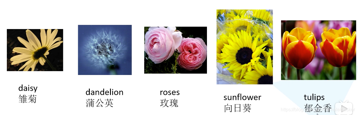
此demo一共包含5个类别的RGB彩色图片。
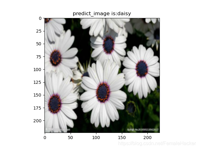
分类测试
【1】daisy

【2】dandelion
在这里插入图片描述
【4】rose
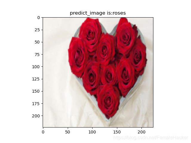

- 玫瑰花因未绽开,所以被识别为郁金香。
【4】sunflowers


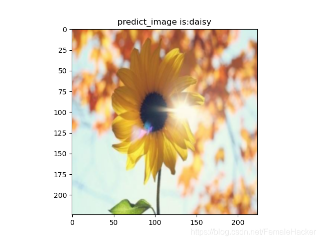
- 向日葵被识别成daisy(菊花)