线代notes_1: MIT18.06 L1-L5

Intro

n linear equations, n unknowns.
E.g:
$$\begin{array}{r}2x-y=0\\ -x+2y=3\end{array}$$
can be written as:
$$\left[\begin{array}{cc}2& -1\\ -1& 2\end{array}\right]\left[\begin{array}{c}x\\ y\end{array}\right]=\left[\begin{array}{c}0\\ 3\end{array}\right]$$
$$AX=b$$

Row picture

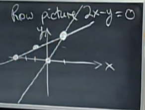
solution: $x=1,y=2$

Column Picture

$$x\left[\begin{array}{c}2\\ -1\end{array}\right]+y\left[\begin{array}{c}-1\\ 2\end{array}\right]=\left[\begin{array}{c}0\\ 3\end{array}\right]$$
to find a linear combination of the columns to produce the new one.

Three variables

$$\begin{array}{r}2x-y=0\\ -x+2y-z=3\\ -3y+4z=4\end{array}$$
$$A=\left[\begin{array}{ccc}2& -1& 0\\ -1& 2& -1\\ 0& -3& 4\end{array}\right]$$

Row picture

Three planes will cross at one point

Column picture

$$x\left[\begin{array}{c}2\\ -1\\ 0\end{array}\right]+y\left[\begin{array}{c}-1\\ 2\\ 3\end{array}\right]+z\left[\begin{array}{c}0\\ -1\\ 4\end{array}\right]=\left[\begin{array}{c}0\\ -1\\ 4\end{array}\right]$$
Can I solve $AX=b$ for every $b$?
=
Do the linear combs of the columns fill 3-D space?

If the 3 column vectors are in the same plane, their linear combinations cannot produce $b$ which is not in this plane.

Singular = not invertible

Lecture 2 Elimination

$A=\left[\begin{array}{ccc}1& 2& 1\\ 3& 8& 1\\ 0& 4& 1\end{array}\right]->\left[\begin{array}{ccc}1& 2& 1\\ 0& 2& -2\\ 0& 4& 1\end{array}\right]->\left[\begin{array}{ccc}1& 2& 1\\ 0& 2& -2\\ 0& 0& 5\end{array}\right]$

Augmented Matrix: Take $b$ to the right side of A.

Row operation
$\left[\begin{array}{cc}a& b\end{array}\right]\left[\begin{array}{cc}c& d\\ e& f\end{array}\right]=a\left[\begin{array}{cc}c& d\end{array}\right]+b\left[\begin{array}{cc}e& f\end{array}\right]$

The elimination process:

$\left[\begin{array}{ccc}1& 0& 0\\ 0& 1& 0\\ 0& -2& 1\end{array}\right]\left[\begin{array}{ccc}1& 0& 0\\ -3& 1& 0\\ 0& 0& 1\end{array}\right]\left[\begin{array}{ccc}1& 2& 1\\ 3& 8& 1\\ 0& 4& 1\end{array}\right]$
Left multiplication means row operation.
Right multiplication means column operation

Lecture 3 Matrix multiplication and Inverses

Inverses

if $A^{-1}$ exists, $A^{-1}A=I$

Invertible = nonsingular

If I can find a non-zero vector $X$ with $AX=0$
a little proof:

$$\begin{gathered} AX=0 \\ {A}^{-1}AX=A^{-1}0=0 \\ X=0 \\ contradictswithnon-zero \end{gathered}$$

Gauss-Jordan

Assume that a row operation is $P$
if $PA=I$, then $PI=A^{-1}$

$P[AI]=[I{A}^{-1}]$

Lecture 4

$(AB{)}^{-1}=B^{-1}{A}^{-1}$
$(A^T{)}^{-1}=(A^{-1}{)}^T$

LU decomposition

$$\left[\begin{array}{cc}1& 0\\ -4& 1\end{array}\right]\left[\begin{array}{cc}2& 1\\ 8& 7\end{array}\right]=\left[\begin{array}{cc}2& 1\\ 0& 3\end{array}\right]$$
$$\left[\begin{array}{cc}2& 1\\ 8& 7\end{array}\right]=\left[\begin{array}{cc}1& 0\\ 4& 1\end{array}\right]\left[\begin{array}{cc}2& 1\\ 0& 3\end{array}\right]$$
$A=LU$

Lecture 5: Permutations

$PA=LU$
$P$: Identity matrix with reordered rows
$P^{-1}=P^T$
$R^{T}R$ is always symmetric:
$$(R^{T}R{)}^T=R^T{R}^{TT}=R^{T}R$$

Vector Space

Additivity and number multiplication.
Every vector space needs the Origin.
$R^n$ = all vectors with n real components.
We can multiply, we can add, and we stay in this vector space.

A line passing 0 is a subspace of $R^2$