目录
说明:
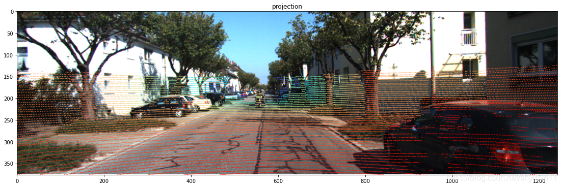
- 将kitti数据集中 雷达点云图像投影到camera图像平面,
- 并生成 深度图的灰度图(灰度值=深度x256 保存成int16位图像(kitti中 depth benchmark的做法))
输入:
- P_rect_02: camera02相机内参
-
R_rect_00: 3x3 纠正旋转矩阵(使图像平面共面)(kitti特有的)
- Tr_velo_to_cam: 激光雷达到camera00的变换矩阵
输出:
- 投影图
- 深度图的灰度图
坐标系:
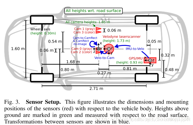
变换公式:
以下等式说明了如何使用齐次坐标在相机0的图像平面上将空间中的3D激光雷达点X投影到2D像素点Y(使用Kitti自述文件中的表示法):

RT_velo_to_cam * x:是将Velodyne坐标中的点x投影到编号为0的相机(参考相机)坐标系中R_rect00 *RT_velo_to_cam * x:是将Velodyne坐标中的点x投影到编号为0的相机(参考相机)坐标系中, 再以参考相机0为基础进行图像共面对齐修正(这是使用KITTI数据集的进行3D投影的必要操作)P_rect_00 * R_rect00 *RT_velo_to_cam * x:是将Velodyne坐标中的点x投影到编号为0的相机(参考相机)坐标系中, 再进行图像共面对齐修正, 然后投影到相机0的像素坐标系中. 如果将P_rect_00改成P_rect_2, 也就是从参考相机0投影到相机2的像素坐标系中(其他相机相对与相机0有偏移b(i)).- 原始论文: Vision meets Robotics: The KITTI Dataset
代码:
# -*- coding: utf-8 -*-

#  数据来源: calib_cam_to_cam.txt
#  下载链接: http://www.cvlibs.net/datasets/kitti/raw_data.php?type=road  >  2011_10_03_drive_0047  >  [calibration]
# R_rect_00: 9.999454e-01 7.259129e-03 -7.519551e-03 -7.292213e-03 9.999638e-01 -4.381729e-03 7.487471e-03 4.436324e-03 9.999621e-01
## P_rect_00: 7.188560e+02 0.000000e+00 6.071928e+02 0.000000e+00 0.000000e+00 7.188560e+02 1.852157e+02 0.000000e+00 0.000000e+00 0.000000e+00 1.000000e+00 0.000000e+00
# ...
## R_rect_02: 9.999191e-01 1.228161e-02 -3.316013e-03 -1.228209e-02 9.999246e-01 -1.245511e-04 3.314233e-03 1.652686e-04 9.999945e-01
# P_rect_02: 7.188560e+02 0.000000e+00 6.071928e+02 4.538225e+01 0.000000e+00 7.188560e+02 1.852157e+02 -1.130887e-01 0.000000e+00 0.000000e+00 1.000000e+00 3.779761e-03

#  数据来源: calib_velo_to_cam.txt
#  下载链接: http://www.cvlibs.net/datasets/kitti/raw_data.php?type=road  >  2011_10_03_drive_0047  >  [calibration]
#   calib_time: 15-Mar-2012 11:45:23
#   R: 7.967514e-03 -9.999679e-01 -8.462264e-04 -2.771053e-03 8.241710e-04 -9.999958e-01 9.999644e-01 7.969825e-03 -2.764397e-03
#   T: -1.377769e-02 -5.542117e-02 -2.918589e-01


# # png bin来源
# data_odometry_color/dataset/sequences/00/image_2
# data_odometry_velodyne/dataset/sequences/00/velodyne

import sys
import matplotlib.pyplot as plt
import matplotlib.image as mpimg
import numpy as np
import utils
from PIL import Image
import math


#-----------------------------------相机02内参矩阵-----------------------------------
P_rect_02 = np.array( [ 7.188560000000e+02, 0.000000000000e+00, 6.071928000000e+02, 4.538225000000e+01,
                                                0.000000000000e+00,7.188560000000e+02, 1.852157000000e+02, -1.130887000000e-01,
                                                0.000000000000e+00, 0.000000000000e+00, 1.000000000000e+00, 3.779761000000e-03]).reshape((3,4))

R_rect_00 = np.array( [ 9.999454e-01, 7.259129e-03, -7.519551e-03,
                                                -7.292213e-03, 9.999638e-01, -4.381729e-03,
                                                7.487471e-03, 4.436324e-03, 9.999621e-01]).reshape((3,3))

# R_rect_02 = np.array( [ 9.999191e-01, 1.228161e-02 -3,.316013e-03,
#                                                 -1.228209e-02, 9.999246e-01, -1.245511e-04,
#                                                 3.314233e-03, 1.652686e-04, 9.999945e-01]).reshape((3,3))


#velo激光雷达 到 相机00(此处已知条件重点注意) 的变换矩阵
Tr_velo_to_cam = np.array( [    7.967514e-03, -9.999679e-01, -8.462264e-04, -1.377769e-02,
                                                                -2.771053e-03, 8.241710e-04, -9.999958e-01, -5.542117e-02,
                                                                9.999644e-01, 7.969825e-03, -2.764397e-03, -2.918589e-01]).reshape((3,4))


#-----------------------------------数据文件位置---------------------------------------
velo_files = "./data/00_velodyne/000005.bin"
rgbimg = "./data/00_image_02/000005.png"
resultImg = "./data/result_merge.png"

data = {}
data['P_rect_20'] = P_rect_02
# Compute the velodyne to rectified camera coordinate transforms
data['T_cam0_velo'] = Tr_velo_to_cam
data['T_cam0_velo'] = np.vstack([data['T_cam0_velo'], [0, 0, 0, 1]])

# pattern1:
R_rect_00 = np.insert(R_rect_00,3,values=[0,0,0],axis=0)
R_rect_00 = np.insert(R_rect_00,3,values=[0,0,0,1],axis=1)
data['T_cam2_velo'] = R_rect_00.dot(data['T_cam0_velo']) #雷达 到 相机02的变换矩阵
print(data['T_cam2_velo'])

pointCloud = utils.load_velo_scan(velo_files)   #读取lidar原始数据
points = pointCloud[:, 0:3]                                           # 获取 lidar xyz (front, left, up)
points_homo = np.insert(points,3,1,axis=1).T    # 齐次化,并转置(一列表示一个点(x,y,z,1), 多少列就有多少个点)
points_homo = np.delete(points_homo,np.where(points_homo[0,:]<0),axis=1) #以列为基准, 删除深度x=0的点

proj_lidar = data['P_rect_20'].dot( data['T_cam2_velo'] ).dot(points_homo)  #相机坐标系3D点=相机02内参*雷达到激光的变换矩阵*雷达3D点
cam = np.delete(proj_lidar,np.where(proj_lidar[2,:]<0),axis=1)  #以列为基准, 删除投影图像点中深度z<0(在投影图像后方)的点 #3xN
cam[:2,:] /= cam[2,:]   # 等价写法 cam[:2] /= cam[2] # 前两行元素分布除以第三行元素(归一化到相机坐标系z=1平面)(x=x/z, y =y/z)


# -----------------------------------将激光投影点绘制到图像平面:绘制原图------------------------------------
png = mpimg.imread(rgbimg)
IMG_H,IMG_W,_ = png.shape
plt.figure(figsize=((IMG_W)/72.0,(IMG_H)/72.0),dpi=72.0, tight_layout=True)
# restrict canvas in range
plt.axis([0,IMG_W,IMG_H,0])
# plt.axis('off')
plt.imshow(png) #在画布上画出原图

# filter point out of canvas
u,v,z = cam
u_out = np.logical_or(u<0, u>IMG_W)
v_out = np.logical_or(v<0, v>IMG_H)
outlier = np.logical_or(u_out, v_out)
cam = np.delete(cam,np.where(outlier),axis=1)
# generate color map from depth
u,v,z = cam

# 将激光投影点绘制到图像平面:绘制激光深度散点图
plt.scatter([u],[v],c=[z],cmap='rainbow_r',alpha=0.5,s=1)
plt.title("projection")
plt.savefig(resultImg,bbox_inches='tight')
plt.show()  #在画布上画出散点雷达深度投影


#-----------------------------------单独保存深度图像成灰度图像---------------------------------------------------
image_array = np.zeros((IMG_H, IMG_W), dtype=np.int16)
for i in range(cam.shape[1]):
    x = int(round(u[i]))
    y = int(round(v[i]))

    # x = math.ceil(u[i]) #向上取整
    # y = math.ceil(v[i])

    depth =  int(z[i]*256)
    if 0<x<image_array.shape[1] and 0<y<image_array.shape[0]:
        image_array[y,x] = depth

image_pil = Image.fromarray(image_array, 'I;16')
image_pil.save("result_16.png")


print("done")
结果:

参考:
- https://github.com/azureology/kitti-velo2cam
- python3.6 > sit-packages>pykitti>odometry.py