转载地址:http://blog.csdn.net/google19890102/article/details/51030884
一、Mean Shift算法概述
Mean Shift算法,又称为均值漂移算法,Mean Shift的概念最早是由Fukunage在1975年提出的,在后来由Yizong Cheng对其进行扩充,主要提出了两点的改进:
核函数的定义使得偏移值对偏移向量的贡献随之样本与被偏移点的距离的不同而不同。权重系数使得不同样本的权重不同。Mean Shift算法在聚类,图像平滑、分割以及视频跟踪等方面有广泛的应用。
二、Mean Shift算法的核心原理
2.1、核函数
在Mean Shift算法中引入核函数的目的是使得随着样本与被偏移点的距离不同,其偏移量对均值偏移向量的贡献也不同。核函数是机器学习中常用的一种方式。核函数的定义如下所示:
X
表示一个
d
维的欧式空间,
x
是该空间中的一个点
x={x1,x2,x3⋯,xd}
,其中,
x
的模
∥x∥2=xxT
,
R
表示实数域,如果一个函数
K:X→R
存在一个剖面函数
k:[0,∞]→R
,即
K(x)=k(∥x∥2)
并且满足:
(1)、
k
是非负的
(2)、
k
是非增的
(3)、
k
是分段连续的
那么,函数
K(x)
就称为核函数。
常用的核函数有高斯核函数。高斯核函数如下所示:
N(x)=12π−−√he−x22h2
其中,
h
称为带宽(bandwidth),不同带宽的核函数如下图所示:
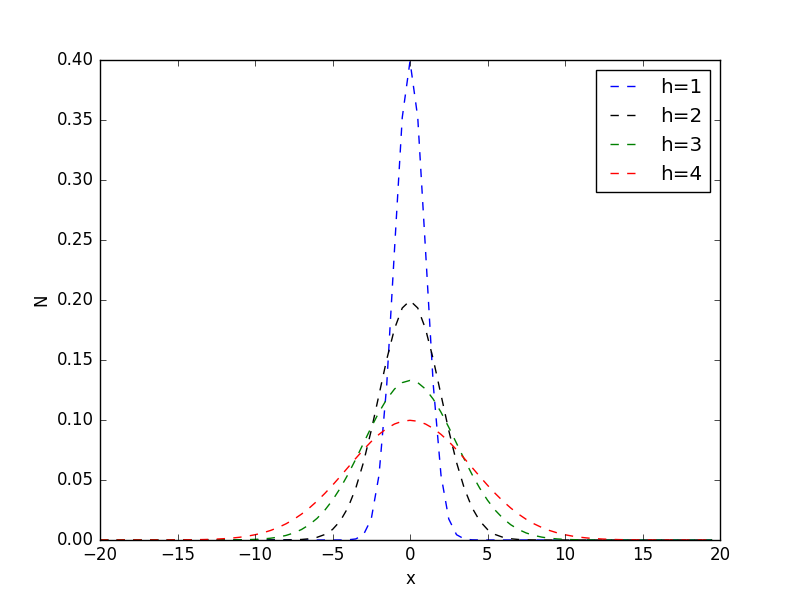
上图的画图脚本如下所示:
'''
Date:201604026
@author: zhaozhiyong
'''
import matplotlib.pyplot as plt
import math

def cal_Gaussian(x, h=1):
    molecule = x * x
    denominator = 2 * h * h
    left = 1 / (math.sqrt(2 * math.pi) * h)
    return left * math.exp(-molecule / denominator)

x = []

for i in xrange(-40,40):
    x.append(i * 0.5);

score_1 = []
score_2 = []
score_3 = []
score_4 = []

for i in x:
    score_1.append(cal_Gaussian(i,1))
    score_2.append(cal_Gaussian(i,2))
    score_3.append(cal_Gaussian(i,3))
    score_4.append(cal_Gaussian(i,4))

plt.plot(x, score_1, 'b--', label="h=1")
plt.plot(x, score_2, 'k--', label="h=2")
plt.plot(x, score_3, 'g--', label="h=3")
plt.plot(x, score_4, 'r--', label="h=4")

plt.legend(loc="upper right")
plt.xlabel("x")
plt.ylabel("N")
plt.show()
- 1
- 2
- 3
- 4
- 5
- 6
- 7
- 8
- 9
- 10
- 11
- 12
- 13
- 14
- 15
- 16
- 17
- 18
- 19
- 20
- 21
- 22
- 23
- 24
- 25
- 26
- 27
- 28
- 29
- 30
- 31
- 32
- 33
- 34
- 35
- 36
- 37
- 38
- 39
- 1
- 2
- 3
- 4
- 5
- 6
- 7
- 8
- 9
- 10
- 11
- 12
- 13
- 14
- 15
- 16
- 17
- 18
- 19
- 20
- 21
- 22
- 23
- 24
- 25
- 26
- 27
- 28
- 29
- 30
- 31
- 32
- 33
- 34
- 35
- 36
- 37
- 38
- 39
2.2、Mean Shift算法的核心思想
2.2.1、基本原理
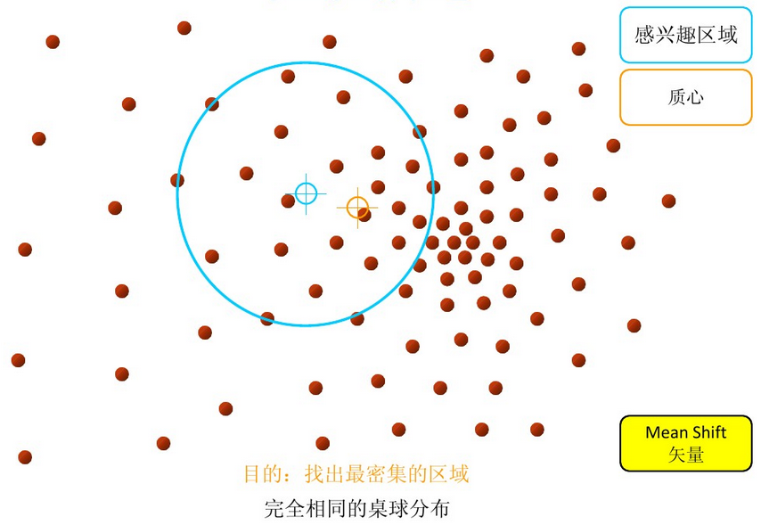
对于Mean Shift算法,是一个迭代的步骤,即先算出当前点的偏移均值,将该点移动到此偏移均值,然后以此为新的起始点,继续移动,直到满足最终的条件。此过程可由下图的过程进行说明(图片来自参考文献3):
- 步骤1:在指定的区域内计算偏移均值(如下图的黄色的圈)
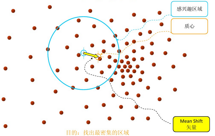
- 步骤3: 重复上述的过程(计算新的偏移均值,移动)
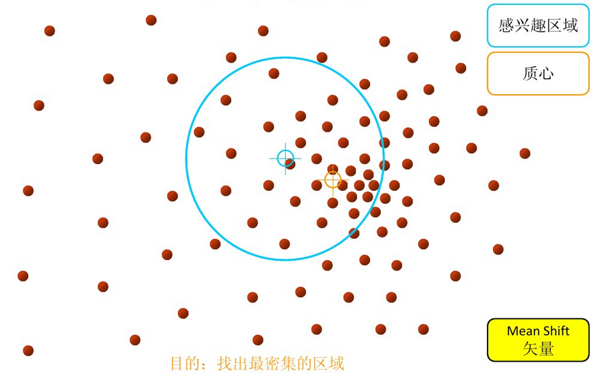
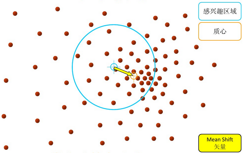
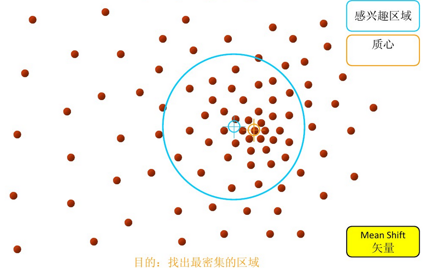
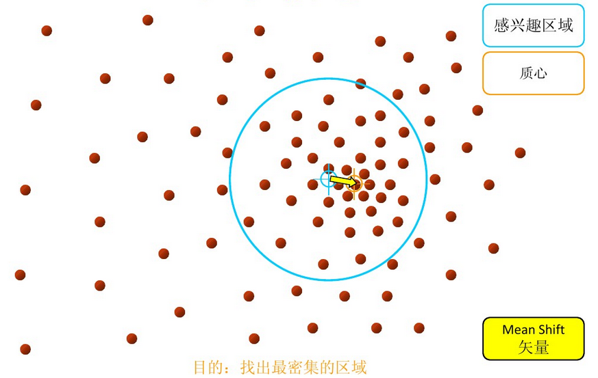
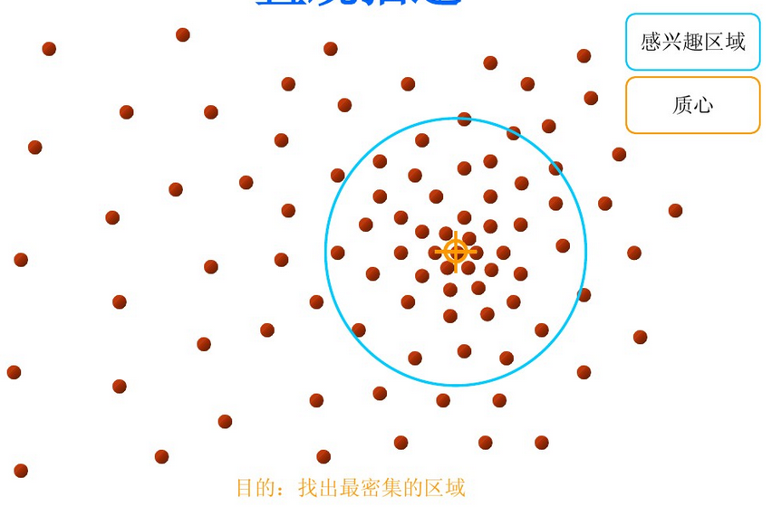
从上述过程可以看出,在Mean Shift算法中,最关键的就是计算每个点的偏移均值,然后根据新计算的偏移均值更新点的位置。
2.2.2、基本的Mean Shift向量形式
对于给定的
d
维空间
Rd
中的
n
个样本点
xi,i=1,⋯,n
,则对于
x
点,其Mean Shift向量的基本形式为:
Mh(x)=1k∑xi∈Sh(xi−x)
其中,
Sh
指的是一个半径为
h
的高维球区域,如上图中的蓝色的圆形区域。
Sh
的定义为:
Sh(x)=(y∣(y−x)(y−x)T⩽h2)
这样的一种基本的Mean Shift形式存在一个问题:在
Sh
的区域内,每一个点对
x
的贡献是一样的。而实际上,这种贡献与
x
到每一个点之间的距离是相关的。同时,对于每一个样本,其重要程度也是不一样的。
2.2.3、改进的Mean Shift向量形式
基于以上的考虑,对基本的Mean Shift向量形式中增加核函数和样本权重,得到如下的改进的Mean Shift向量形式:
Mh(x)=∑ni=1GH(xi−x)w(xi)(xi−x)∑ni=1GH(xi−x)w(xi)
其中:
GH(xi−x)=|H|−12G(H−12(xi−x))
G(x)
是一个单位的核函数。
H
是一个正定的对称
d×d
矩阵,称为带宽矩阵,其是一个对角阵。
w(xi)⩾0
是每一个样本的权重。对角阵
H
的形式为:
H=⎛⎝⎜⎜⎜⎜⎜h210⋮00h22⋮0⋯⋯⋯00⋮h2d⎞⎠⎟⎟⎟⎟⎟d×d
上述的Mean Shift向量可以改写成:
Mh(x)=∑ni=1G(xi−xhi)w(xi)(xi−x)∑ni=1G(xi−xhi)w(xi)
Mean Shift向量
Mh(x)
是归一化的概率密度梯度。
2.3、Mean Shift算法的解释
在Mean Shift算法中,实际上是利用了概率密度,求得概率密度的局部最优解。
2.3.1、概率密度梯度
对一个概率密度函数
f(x)
,已知
d
维空间中
n
个采样点
xi,i=1,⋯,n
,
f(x)
的核函数估计(也称为Parzen窗估计)为:
f^(x)=∑ni=1K(xi−xh)w(xi)hd∑ni=1w(xi)
其中
w(xi)⩾0
是一个赋给采样点
xi
的权重
K(x)
是一个核函数
概率密度函数
f(x)
的梯度
▽f(x)
的估计为
▽f^(x)=2∑ni=1(x−xi)k′(∥∥xi−xh∥∥2)w(xi)hd+2∑ni=1w(xi)
令
g(x)=−k′(x)
,
G(x)=g(∥x∥2)
,则有:
▽f^(x)=2∑ni=1(xi−x)G(∥∥xi−xh∥∥2)w(xi)hd+2∑ni=1w(xi)=2h2⎡⎣⎢∑ni=1G(xi−xh)w(xi)hd∑ni=1w(xi)⎤⎦⎥⎡⎣⎢∑ni=1(xi−x)G(∥∥xi−xh∥∥2)w(xi)∑ni=1G(xi−xh)w(xi)⎤⎦⎥
其中,第二个方括号中的就是Mean Shift向量,其与概率密度梯度成正比。
2.3.2、Mean Shift向量的修正
Mh(x)=∑ni=1G(∥∥xi−xh∥∥2)w(xi)xi∑ni=1G(xi−xh)w(xi)−x
记:
mh(x)=∑ni=1G(∥∥xi−xh∥∥2)w(xi)xi∑ni=1G(xi−xh)w(xi)
,则上式变成:
Mh(x)=mh(x)+x
这与梯度上升的过程一致。
2.4、Mean Shift算法流程
Mean Shift算法的算法流程如下:
- 计算
mh(x)
- 令
x=mh(x)
- 如果
∥mh(x)−x∥<ε
,结束循环,否则,重复上述步骤
三、实验
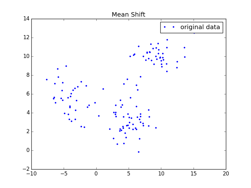
3.1、实验数据
实验数据如下图所示(来自参考文献1):
画图的代码如下:
'''
Date:20160426
@author: zhaozhiyong
'''
import matplotlib.pyplot as plt

f = open("data")
x = []
y = []
for line in f.readlines():
    lines = line.strip().split("\t")
    if len(lines) == 2:
        x.append(float(lines[0]))
        y.append(float(lines[1]))
f.close()

plt.plot(x, y, 'b.', label="original data")
plt.title('Mean Shift')
plt.legend(loc="upper right")
plt.show()
- 1
- 2
- 3
- 4
- 5
- 6
- 7
- 8
- 9
- 10
- 11
- 12
- 13
- 14
- 15
- 16
- 17
- 18
- 19
- 20
- 21
- 1
- 2
- 3
- 4
- 5
- 6
- 7
- 8
- 9
- 10
- 11
- 12
- 13
- 14
- 15
- 16
- 17
- 18
- 19
- 20
- 21
3.2、实验的源码
'''
Date:20160426
@author: zhaozhiyong
'''
import math
import sys
import numpy as np
MIN_DISTANCE = 0.000001
def load_data(path, feature_num=2):
f = open(path)
data = []
for line in f.readlines():
lines = line.strip().split("\t")
data_tmp = []
if len(lines) != feature_num:
continue
for i in xrange(feature_num):
data_tmp.append(float(lines[i]))
data.append(data_tmp)
f.close()
return data
def gaussian_kernel(distance, bandwidth):
m = np.shape(distance)[0]
right = np.mat(np.zeros((m, 1)))
for i in xrange(m):
right[i, 0] = (-0.5 * distance[i] * distance[i].T) / (bandwidth * bandwidth)
right[i, 0] = np.exp(right[i, 0])
left = 1 / (bandwidth * math.sqrt(2 * math.pi))
gaussian_val = left * right
return gaussian_val
def shift_point(point, points, kernel_bandwidth):
points = np.mat(points)
m,n = np.shape(points)
point_distances = np.mat(np.zeros((m,1)))
for i in xrange(m):
point_distances[i, 0] = np.sqrt((point - points[i]) * (point - points[i]).T)
point_weights = gaussian_kernel(point_distances, kernel_bandwidth)
all = 0.0
for i in xrange(m):
all += point_weights[i, 0]
point_shifted = point_weights.T * points / all
return point_shifted
def euclidean_dist(pointA, pointB):
total = (pointA - pointB) * (pointA - pointB).T
return math.sqrt(total)
def distance_to_group(point, group):
min_distance = 10000.0
for pt in group:
dist = euclidean_dist(point, pt)
if dist < min_distance:
min_distance = dist
return min_distance
def group_points(mean_shift_points):
group_assignment = []
m,n = np.shape(mean_shift_points)
index = 0
index_dict = {}
for i in xrange(m):
item = []
for j in xrange(n):
item.append(str(("%5.2f" % mean_shift_points[i, j])))
item_1 = "_".join(item)
print item_1
if item_1 not in index_dict:
index_dict[item_1] = index
index += 1
for i in xrange(m):
item = []
for j in xrange(n):
item.append(str(("%5.2f" % mean_shift_points[i, j])))
item_1 = "_".join(item)
group_assignment.append(index_dict[item_1])
return group_assignment
def train_mean_shift(points, kenel_bandwidth=2):
mean_shift_points = np.mat(points)
max_min_dist = 1
iter = 0
m, n = np.shape(mean_shift_points)
need_shift = [True] * m
while max_min_dist > MIN_DISTANCE:
max_min_dist = 0
iter += 1
print "iter : " + str(iter)
for i in range(0, m):
if not need_shift[i]:
continue
p_new = mean_shift_points[i]
p_new_start = p_new
p_new = shift_point(p_new, points, kenel_bandwidth)
dist = euclidean_dist(p_new, p_new_start)
if dist > max_min_dist:
max_min_dist = dist
if dist < MIN_DISTANCE:
need_shift[i] = False
mean_shift_points[i] = p_new
group = group_points(mean_shift_points)
return np.mat(points), mean_shift_points, group
if __name__ == "__main__":
path = "./data"
data = load_data(path, 2)
points, shift_points, cluster = train_mean_shift(data, 2)
for i in xrange(len(cluster)):
print "%5.2f,%5.2f\t%5.2f,%5.2f\t%i" % (points[i,0], points[i, 1], shift_points[i, 0], shift_points[i, 1], cluster[i])
- 1
- 2
- 3
- 4
- 5
- 6
- 7
- 8
- 9
- 10
- 11
- 12
- 13
- 14
- 15
- 16
- 17
- 18
- 19
- 20
- 21
- 22
- 23
- 24
- 25
- 26
- 27
- 28
- 29
- 30
- 31
- 32
- 33
- 34
- 35
- 36
- 37
- 38
- 39
- 40
- 41
- 42
- 43
- 44
- 45
- 46
- 47
- 48
- 49
- 50
- 51
- 52
- 53
- 54
- 55
- 56
- 57
- 58
- 59
- 60
- 61
- 62
- 63
- 64
- 65
- 66
- 67
- 68
- 69
- 70
- 71
- 72
- 73
- 74
- 75
- 76
- 77
- 78
- 79
- 80
- 81
- 82
- 83
- 84
- 85
- 86
- 87
- 88
- 89
- 90
- 91
- 92
- 93
- 94
- 95
- 96
- 97
- 98
- 99
- 100
- 101
- 102
- 103
- 104
- 105
- 106
- 107
- 108
- 109
- 110
- 111
- 112
- 113
- 114
- 115
- 116
- 117
- 118
- 119
- 120
- 121
- 122
- 123
- 124
- 125
- 126
- 127
- 128
- 129
- 130
- 131
- 132
- 133
- 134
- 135
- 136
- 137
- 138
- 139
- 140
- 141
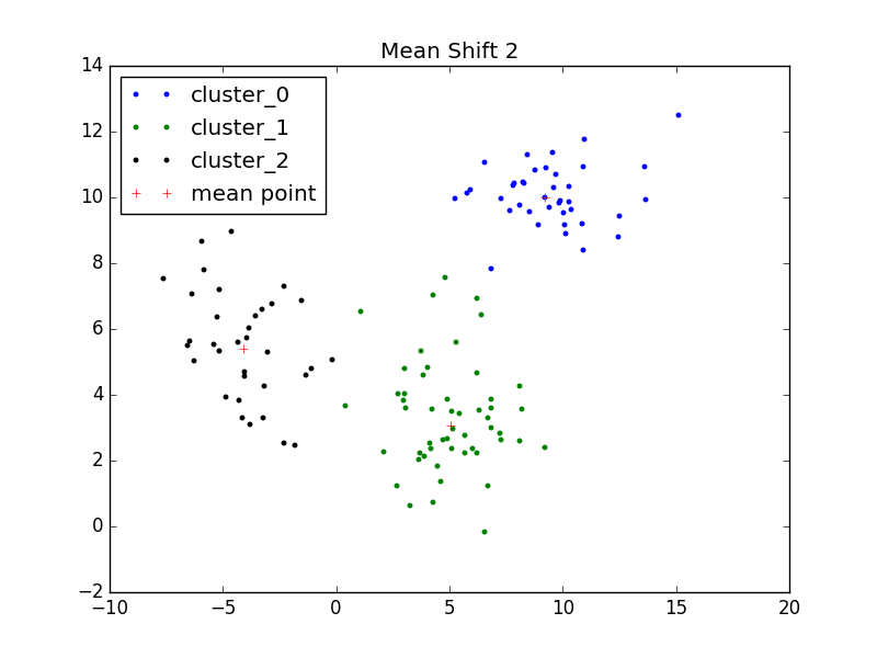
3.3、实验的结果
经过Mean Shift算法聚类后的数据如下所示:
'''
Date:20160426
@author: zhaozhiyong
'''
import matplotlib.pyplot as plt

f = open("data_mean")
cluster_x_0 = []
cluster_x_1 = []
cluster_x_2 = []
cluster_y_0 = []
cluster_y_1 = []
cluster_y_2 = []
center_x = []
center_y = []
center_dict = {}

for line in f.readlines():
    lines = line.strip().split("\t")
    if len(lines) == 3:
        label = int(lines[2])
        if label == 0:
            data_1 = lines[0].strip().split(",")
            cluster_x_0.append(float(data_1[0]))
            cluster_y_0.append(float(data_1[1]))
            if label not in center_dict:
                center_dict[label] = 1
                data_2 = lines[1].strip().split(",")
                center_x.append(float(data_2[0]))
                center_y.append(float(data_2[1]))
        elif label == 1:
            data_1 = lines[0].strip().split(",")
            cluster_x_1.append(float(data_1[0]))
            cluster_y_1.append(float(data_1[1]))
            if label not in center_dict:
                center_dict[label] = 1
                data_2 = lines[1].strip().split(",")
                center_x.append(float(data_2[0]))
                center_y.append(float(data_2[1]))
        else:
            data_1 = lines[0].strip().split(",")
            cluster_x_2.append(float(data_1[0]))
            cluster_y_2.append(float(data_1[1]))
            if label not in center_dict:
                center_dict[label] = 1
                data_2 = lines[1].strip().split(",")
                center_x.append(float(data_2[0]))
                center_y.append(float(data_2[1]))
f.close()


plt.plot(cluster_x_0, cluster_y_0, 'b.', label="cluster_0")
plt.plot(cluster_x_1, cluster_y_1, 'g.', label="cluster_1")
plt.plot(cluster_x_2, cluster_y_2, 'k.', label="cluster_2")
plt.plot(center_x, center_y, 'r+', label="mean point")
plt.title('Mean Shift 2')
#plt.legend(loc="best")
plt.show()
- 1
- 2
- 3
- 4
- 5
- 6
- 7
- 8
- 9
- 10
- 11
- 12
- 13
- 14
- 15
- 16
- 17
- 18
- 19
- 20
- 21
- 22
- 23
- 24
- 25
- 26
- 27
- 28
- 29
- 30
- 31
- 32
- 33
- 34
- 35
- 36
- 37
- 38
- 39
- 40
- 41
- 42
- 43
- 44
- 45
- 46
- 47
- 48
- 49
- 50
- 51
- 52
- 53
- 54
- 55
- 56
- 57
- 58
- 1
- 2
- 3
- 4
- 5
- 6
- 7
- 8
- 9
- 10
- 11
- 12
- 13
- 14
- 15
- 16
- 17
- 18
- 19
- 20
- 21
- 22
- 23
- 24
- 25
- 26
- 27
- 28
- 29
- 30
- 31
- 32
- 33
- 34
- 35
- 36
- 37
- 38
- 39
- 40
- 41
- 42
- 43
- 44
- 45
- 46
- 47
- 48
- 49
- 50
- 51
- 52
- 53
- 54
- 55
- 56
- 57
- 58
参考文献
-
Mean Shift Clustering
-
Meanshift,聚类算法
-
meanshift算法简介