深度学习之卷积网络手写数字图片识别案例

注意：

该程序运行环境为：pycharm2020+python3.7+tensorflow2.2 cpu版本

因为在学习的过程时，学习视频使用的是tensorflow2.x以下的版本，所以在运行中出现了许多错误，不过已经更正。下面代码都可正常运行。需注意的是：

当导入mnist数据集时会报出
ModuleNotFoundError: No module named ‘tensorflow.examples.tutorials’ 错误

原因是tensorflow_core中缺tutorial文件夹

解决办法就是下载缺失的tutorial文件夹放到 tensorflow_core 目录下

但是tensorflow2.2可能找不到tensorflow_core，这是因为2.2版本将core合并到tensorflow，所以，将下载好的tutorial文件夹放在tensorflow的examples里即可，下载地址如下：tutorial文件夹

1、Mnist数字识别卷积实现案例

1.1 题干分析

1.1.1 参数计算

卷积神经⽹络：

• ⼀卷积层：卷积：32个filter, 5*5，strides1, padding=“SAME” bias = 32

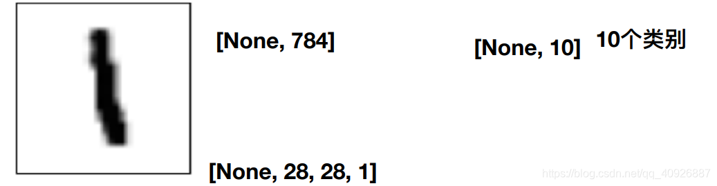
  • 输⼊：[None, 28, 28, 1] 输出：[None, 28,28, 32]

  • 激活:[None, 28,28, 32]

  • 池化：2*2 ,strides2, padding=“SAME”

  • 池化过程的输入输出结果： [None, 28, 28, 32]———>[None, 14, 14, 32]

• ⼆卷积层：卷积:64个filter，5*5，strides1,padding=“SAME” bias = 64

  • 输⼊：[None, 14, 14, 32] 输出：[None, 14, 14, 64]

  • 激活:[None, 14, 14, 64]

  • 池化:2*2， strides2

  • 池化过程的输入输出结果： 输⼊：[None, 14, 14, 64] 输出：[None, 7, 7, 64]

• 全连接层FC：bias = 10

  • [None, 28, 28, 1]
  • 输入：[None, 7x7x64]———> 权重 ：[7x7x64, 10] ———> 结果： [None, 10]

注意： ⼀卷积层：输⼊：[None, 28, 28, 1] 输出：[None, 28,28, 32]、其中1为黑白图片的通道数，输出中的32为32个filter观察来的结果即32张表数据。

1.1.2 相关代码

import tensorflow as tf
from tensorflow.examples.tutorials.mnist import input_data
tf.compat.v1.disable_eager_execution()

# 定义一个初始化权重的函数
def weight_variables(shape):
    w = tf.compat.v1.Variable(tf.compat.v1.random.normal(shape=shape, mean=0.0, stddev=1.0))
    return w


# 定义一个初始化偏置的函数
def bias_variables(shape):
    b = tf.compat.v1.Variable(tf.compat.v1.constant(0.0, shape=shape))
    return b


def model():
    """
    自定义的卷积模型
    :return:
    """
    # 1、准备数据的占位符 x [None, 784]  y_true [None, 10]
    with tf.compat.v1.variable_scope("data"):
        x = tf.compat.v1.placeholder(tf.compat.v1.float32, [None, 784])

        y_true = tf.compat.v1.placeholder(tf.compat.v1.int32, [None, 10])

    # 2、一卷积层 卷积: 5*5*1，32个，strides=1 激活: tf.nn.relu 池化
    with tf.compat.v1.variable_scope("conv1"):
        # 随机初始化权重, 偏置[32]
        w_conv1 = weight_variables([5, 5, 1, 32])

        b_conv1 = bias_variables([32])

        # 对x进行形状的改变[None, 784]  [None, 28, 28, 1]
        x_reshape = tf.compat.v1.reshape(x, [-1, 28, 28, 1])    # -1即为None,表示样本的数量未知

        # 使用relu激活函数、[None, 28, 28, 1]-----> [None, 28, 28, 32]
        x_relu1 = tf.compat.v1.nn.relu(tf.compat.v1.nn.conv2d(x_reshape, w_conv1, strides=[1, 1, 1, 1], padding="SAME") + b_conv1)

        # 池化 2*2 ,strides2 [None, 28, 28, 32]---->[None, 14, 14, 32]
        x_pool1 = tf.compat.v1.nn.max_pool(x_relu1, ksize=[1, 2, 2, 1], strides=[1, 2, 2, 1], padding="SAME")

    # 3、二卷积层卷积:【一层输出32张表，二层每人应观察32张5*5】 5*5*32，64个filter，strides=1 激活: tf.nn.relu 池化：
    with tf.compat.v1.variable_scope("conv2"):
        # 随机初始化权重,  权重：[5, 5, 32, 64]  偏置[64]
        w_conv2 = weight_variables([5, 5, 32, 64])

        b_conv2 = bias_variables([64])

        # 卷积，激活，池化计算
        # [None, 14, 14, 32]-----> [None, 14, 14, 64]
        x_relu2 = tf.compat.v1.nn.relu(tf.compat.v1.nn.conv2d(x_pool1, w_conv2, strides=[1, 1, 1, 1], padding="SAME") + b_conv2)

        # 池化 2*2, strides 2, [None, 14, 14, 64]---->[None, 7, 7, 64]
        x_pool2 = tf.compat.v1.nn.max_pool(x_relu2, ksize=[1, 2, 2, 1], strides=[1, 2, 2, 1], padding="SAME")

    # 4、全连接层 [None, 7, 7, 64]--->[None, 7*7*64]*[7*7*64, 10]+ [10] =[None, 10]
    with tf.compat.v1.variable_scope("conv2"):
        # 随机初始化权重和偏置
        w_fc = weight_variables([7 * 7 * 64, 10])

        b_fc = bias_variables([10])

        # 修改形状 [None, 7, 7, 64] --->None, 7*7*64]
        x_fc_reshape = tf.compat.v1.reshape(x_pool2, [-1, 7 * 7 * 64])

        # 进行矩阵运算得出每个样本的10个结果
        y_predict = tf.compat.v1.matmul(x_fc_reshape, w_fc) + b_fc

    return x, y_true, y_predict


def conv_fc():
    # 获取真实的数据
    mnist = input_data.read_data_sets("./data/mnist/input_data/", one_hot=True)

    # 定义模型，得出输出
    x, y_true, y_predict = model()

    # 进行交叉熵损失计算
    # 3、求出所有样本的损失，然后求平均值
    with tf.compat.v1.variable_scope("soft_cross"):
        # 求平均交叉熵损失
        loss = tf.compat.v1.reduce_mean(tf.compat.v1.nn.softmax_cross_entropy_with_logits(labels=y_true, logits=y_predict))

    # 4、梯度下降求出损失
    with tf.compat.v1.variable_scope("optimizer"):
        train_op = tf.compat.v1.train.GradientDescentOptimizer(0.0001).minimize(loss)   # 学习率0.0001

    # 5、计算准确率
    with tf.compat.v1.variable_scope("acc"):
        equal_list = tf.compat.v1.equal(tf.compat.v1.argmax(y_true, 1), tf.compat.v1.compat.v1.argmax(y_predict, 1))

        # equal_list  None个样本   [1, 0, 1, 0, 1, 1,..........]
        accuracy = tf.compat.v1.reduce_mean(tf.compat.v1.cast(equal_list, tf.compat.v1.float32))

    # 定义一个初始化变量的op
    init_op = tf.compat.v1.global_variables_initializer()

    # 开启回话运行
    with tf.compat.v1.Session() as sess:
        sess.run(init_op)

        # 循环去训练
        for i in range(2000):
            # 取出真实存在的特征值和目标值
            mnist_x, mnist_y = mnist.train.next_batch(50)

            # 运行train_op训练
            sess.run(train_op, feed_dict={
    
    x: mnist_x, y_true: mnist_y})

            print("训练第%d步,准确率为:%f" % (i, sess.run(accuracy, feed_dict={
    
    x: mnist_x, y_true: mnist_y})))

    return None


if __name__ == "__main__":
    conv_fc()

输出的结果：训练第0步,准确率为:0.100000
训练第1步,准确率为:0.080000
训练第2步,准确率为:0.080000
训练第3步,准确率为:0.040000
训练第4步,准确率为:0.120000
训练第5步,准确率为:0.080000
训练第6步,准确率为:0.060000
训练第7步,准确率为:0.080000
训练第8步,准确率为:0.080000
训练第9步,准确率为:0.060000
..........
训练第1990步,准确率为:0.860000
训练第1991步,准确率为:0.860000
训练第1992步,准确率为:0.760000
训练第1993步,准确率为:0.840000
训练第1994步,准确率为:0.820000
训练第1995步,准确率为:0.780000
训练第1996步,准确率为:0.880000
训练第1997步,准确率为:0.820000
训练第1998步,准确率为:0.860000
训练第1999步,准确率为:0.740000

注意： 结果中准确率出现较大幅度的浮动，是因为学习率设置过大的原因造成的。

2、 常见卷积网络模型的结构