多目标跟踪(Multiple Object Tracking)简称MOT,在每个视频帧都要定位目标,并且绘制出他们的轨迹。
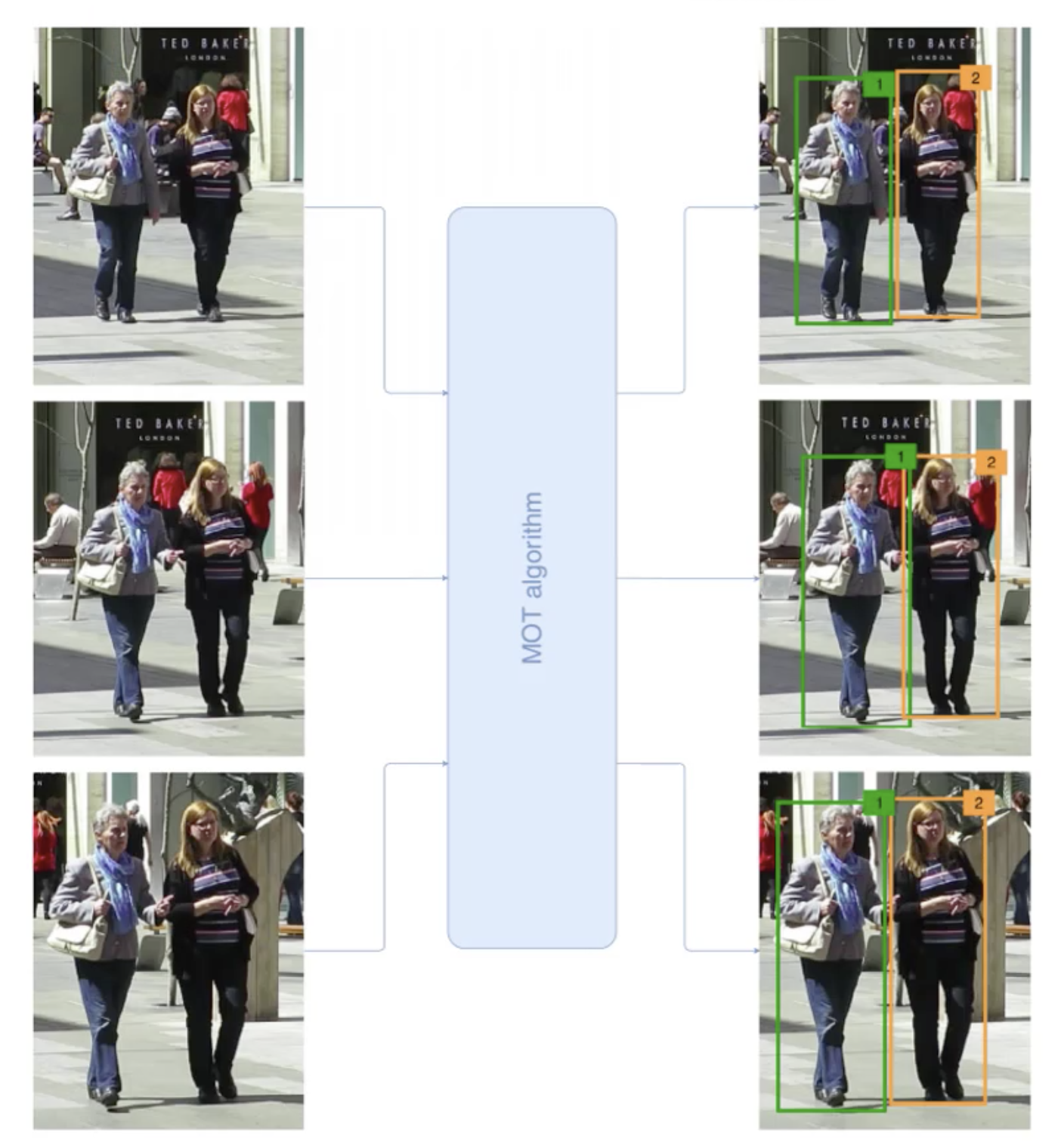
它的输入是视频序列,输出为对于每一个目标的轨迹以及唯一识别ID,也就是说对于不同帧,我们不仅仅要识别出目标(带目标框),而且需要对每一个目标标识一个ID来进行前后帧的关联。
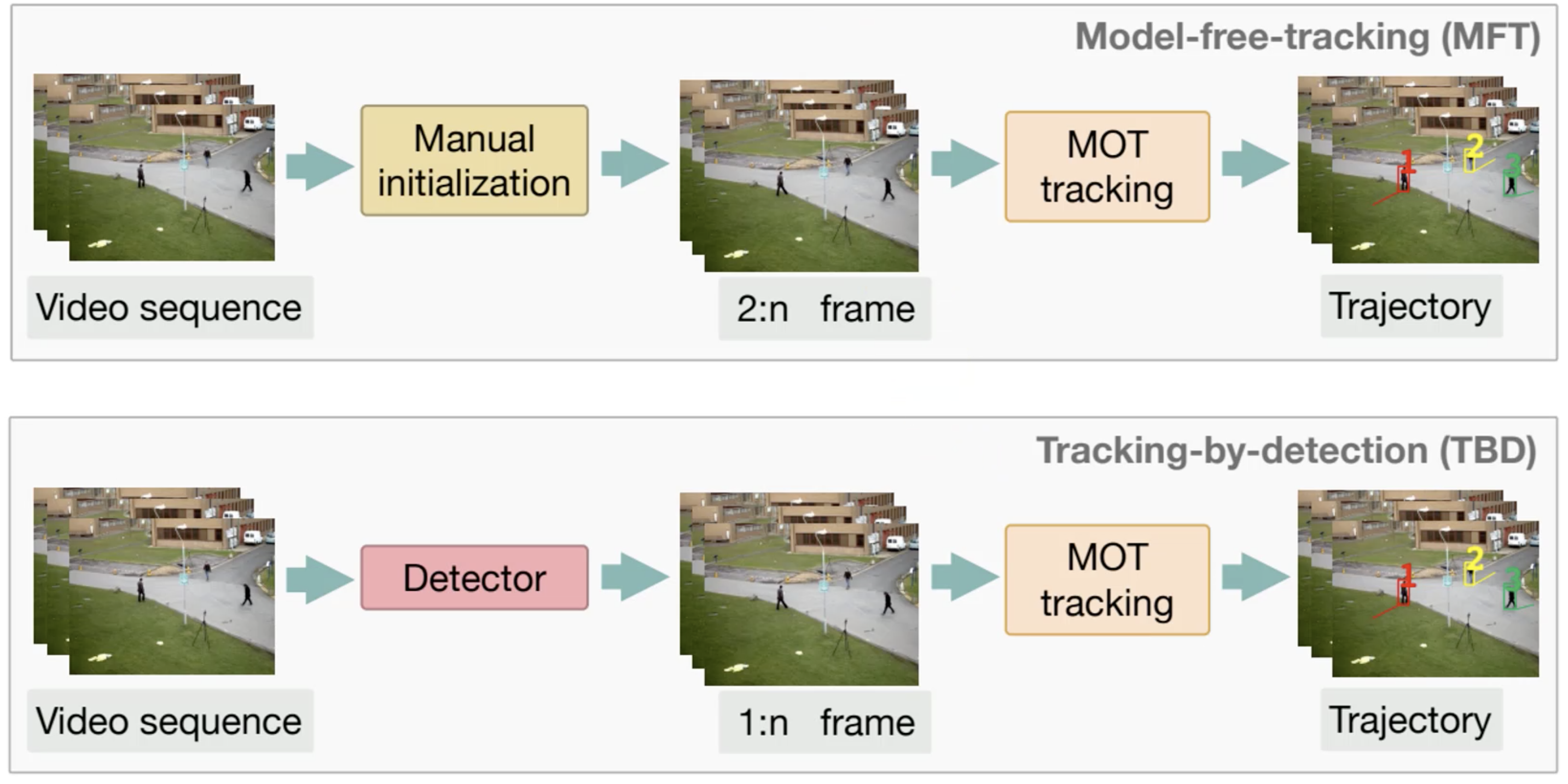
多目标跟踪的技术有两个划分,一个是Model-free-tracking(MFT),它需要做手工的初始化,需要在第一帧标记需要跟踪哪些行人,在后面的帧中做多目标跟踪,得到每一个人运行的轨迹。另一个是Tracking-by-deection(TBD),它不需要在第一帧中指定,在任何一帧中都是使用检测器来检测出视频帧中有几个行人,并且进行多目标跟踪来得到行人轨迹。这里我们主要使用的是第二种TBD技术。
TBD技术的过程如下:
- 对视频帧进行分割
- 使用目标检测网络对目标进行检测(我们这里使用的是YOLOV5)
- 在前后帧对于检测目标的属性做一定的匹配,属性主要包括人的外观特征。这个过程类似于人脸匹配,提取特征,计算相似度。
- 给匹配上的目标使用相同的ID。

算法流程
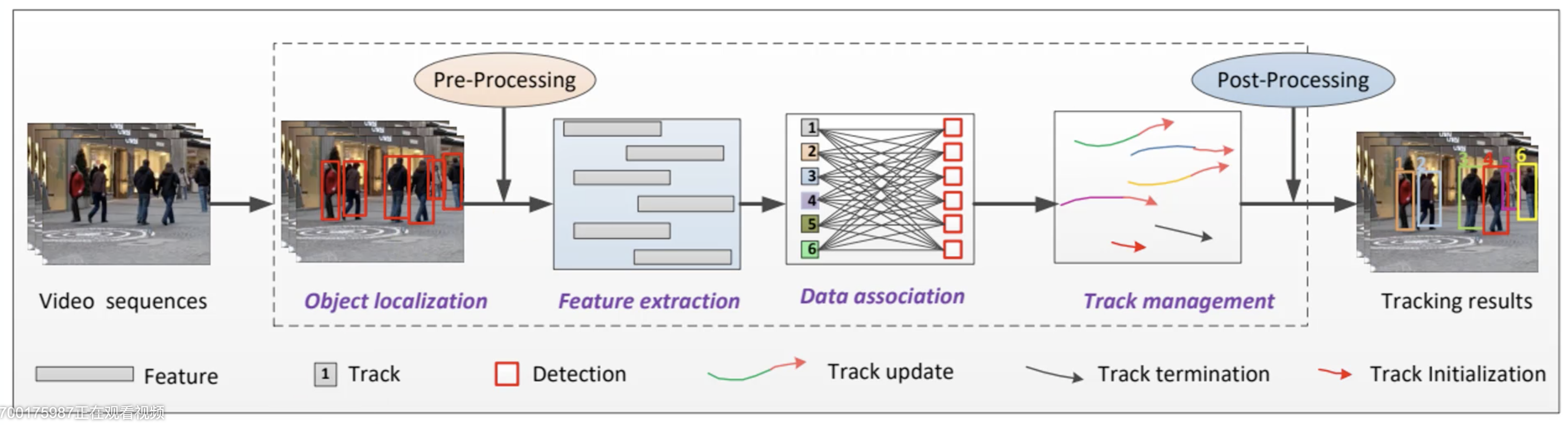
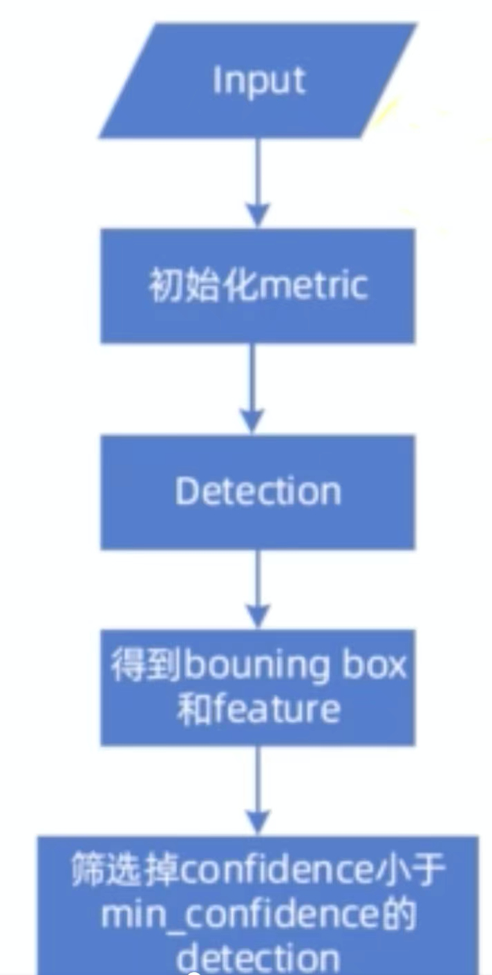
这里对于输入的视频帧进行目标检测,通过预处理(非极大值抑制、置信度过滤器)提取特征,再经过数据关联(Data association),再进行轨迹管理(Track management,包括轨迹更新,轨迹结束,轨迹初始化),通过后处理(帧匹配阈值),最后得到多目标跟踪的结果。
网络结构

将视频图像送入到卷积层、最大池化层、残差块、全连接层、BATCH+L2归一化。
原理篇
基本原理有3个部分,一是马氏距离,这个在之前Tensorflow的图像操作(二) 中有说过;二是匈牙利算法,这个可以参考图论整理 中的匈牙利算法;这里我们重点看第三个——卡尔曼滤波器(Kalman Filter)。
卡尔曼滤波:利用线性系统状态方程,通过系统输入输出观测数据,对系统状态进行最优估计。卡尔曼提出的递推最优估计理论,采用状态空间描述法,能处理多维和非平稳的随机过程。
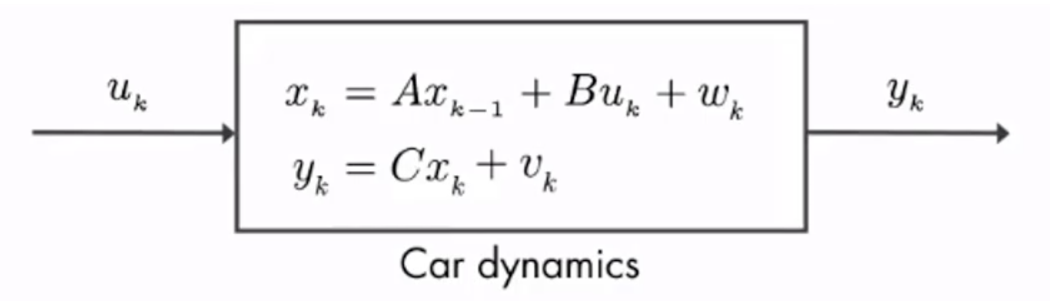
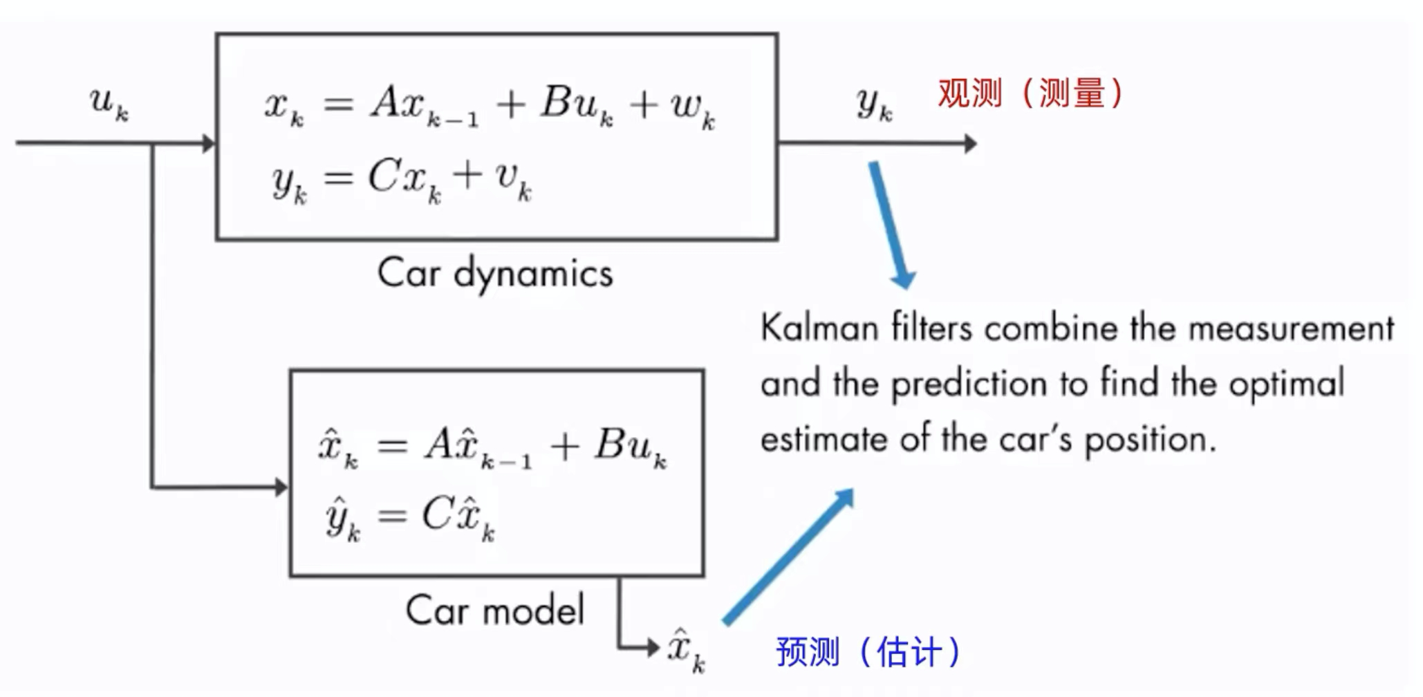
上图是一个车辆动态的线性状态空间表示,![]() 是控制量,比如说踩油门就是一种加速控制;
是控制量,比如说踩油门就是一种加速控制;![]() 是观测值;
是观测值;![]() 是状态,它可以用一个递推式表示,A、B是矩阵,
是状态,它可以用一个递推式表示,A、B是矩阵,![]() 是噪声。在观测值
是噪声。在观测值![]() 中,C是一个矩阵,
中,C是一个矩阵,![]() 是噪声。
是噪声。
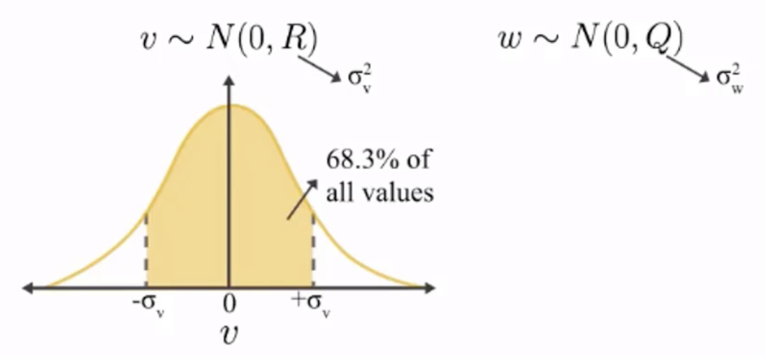
这里我们都默认噪声v和w都服从正态分布,均值为0,方差为R和Q。
在运用中,我们可以有观测值![]() ,或者叫测量值(measurement);还可以有一个预测值
,或者叫测量值(measurement);还可以有一个预测值![]() ,或者叫估计值。我们可以结合观测值和预测值来得到一个更好的估计。那么卡尔曼滤波器就可以结合测量值和预测值来找到一个车辆位置的最优的估计。
,或者叫估计值。我们可以结合观测值和预测值来得到一个更好的估计。那么卡尔曼滤波器就可以结合测量值和预测值来找到一个车辆位置的最优的估计。
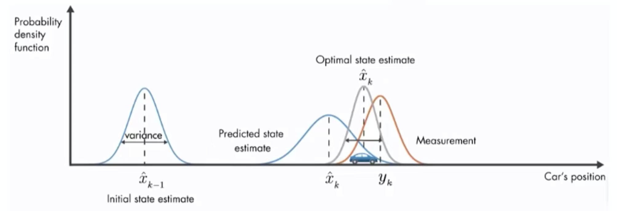
上图中是车辆位置估计图,它的纵坐标为概率密度函数。在开始的时候有一个初始位置估计![]() ,它满足正态分布,经过一段时间之后,有一个估计值
,它满足正态分布,经过一段时间之后,有一个估计值![]() ,和一个观测值
,和一个观测值![]() ,它们俩都满足正态分布,都有均值和方差,都有不确定性。那么怎么得到一个更优的估计呢,那么简单的方法就是将两者进行加权求和。
,它们俩都满足正态分布,都有均值和方差,都有不确定性。那么怎么得到一个更优的估计呢,那么简单的方法就是将两者进行加权求和。
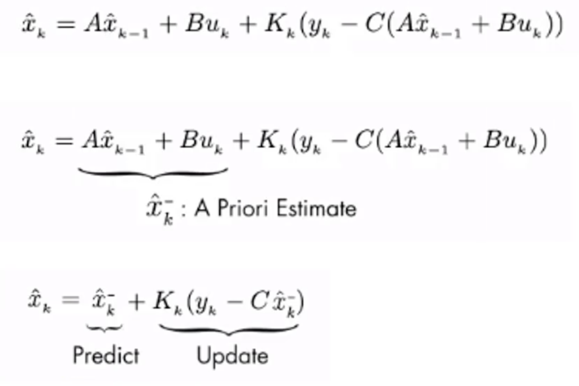
卡尔曼滤波器可以找到估计值和观测值如何进行加权,我们需要通过一个![]() (卡尔曼增益)来结合观测值和估计值。它结合了预测部分(Predict)和观测部分(Update),这两部分的公式如下。
(卡尔曼增益)来结合观测值和估计值。它结合了预测部分(Predict)和观测部分(Update),这两部分的公式如下。
在Update部分,比较关键的就是![]() (卡尔曼增益),我们求出了卡尔曼增益之后,就可以得到新的状态的估计值
(卡尔曼增益),我们求出了卡尔曼增益之后,就可以得到新的状态的估计值![]() ,以及新的状态的协方差估计
,以及新的状态的协方差估计![]() 。
。
它还适用于多传感器融合,比如我们对位置有两个观测值,一个是通过GPS,一个是通过IMU(惯性测量导航)。对这两个Measurement也可以融合在一起,再结合预测值一起来求出最优的估计。
使用时一般忽略u控制输入,得到:

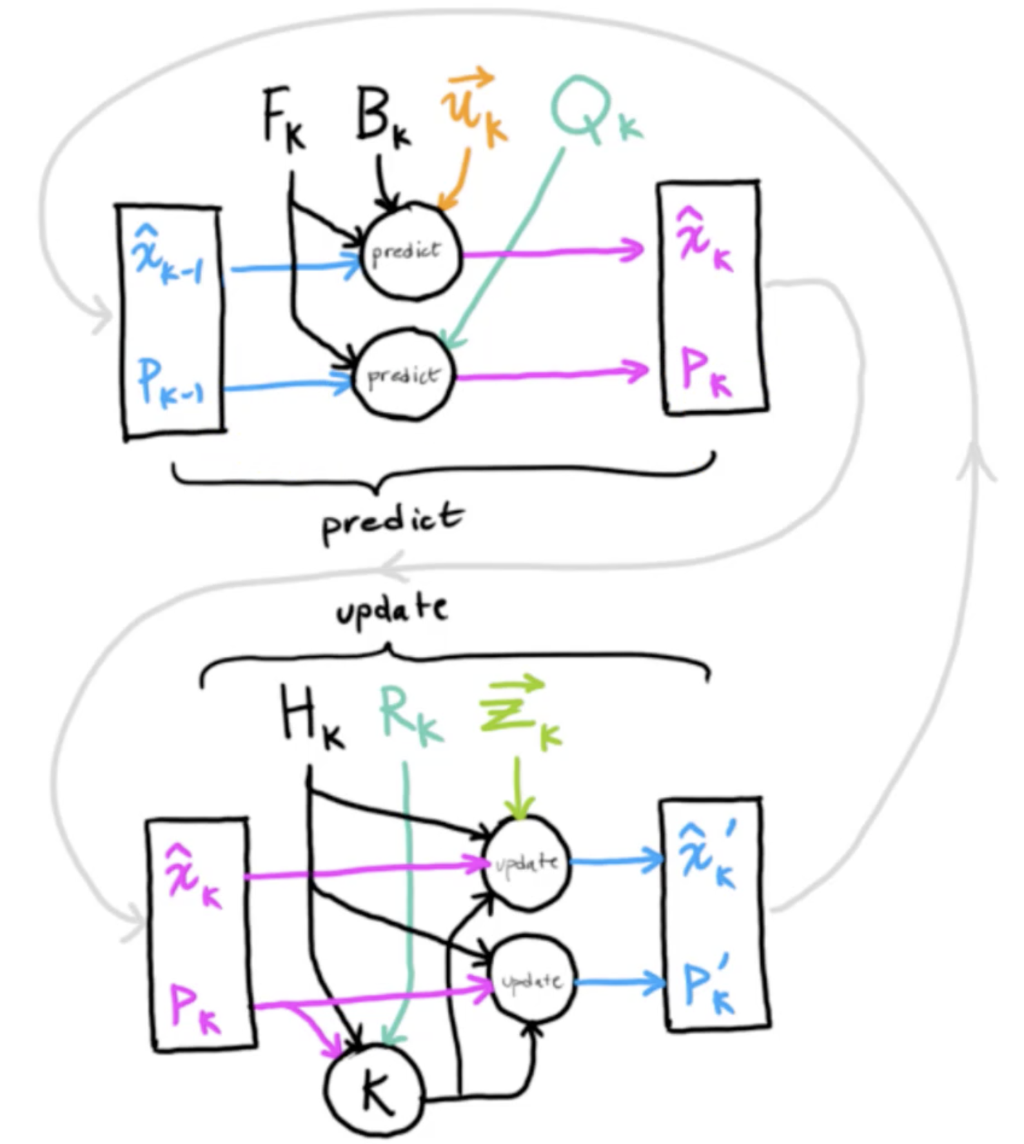
卡尔曼滤波器循环
首先卡尔曼滤波器对于提供的状态信息要进行预测下一个状态,然后结合带有噪声的观测值进行矫正,得到当前状态,然后以此反复。
多目标跟踪的应用
上图中纵坐标是位置,横坐标是速度,它们都满足正态分布,有其均值和方差。位置和速度往往还有关联,所以我们可以求它们的协方差。
我们做预测的话,首先可以做状态预测,新的最优估计是根据上一最优估计预测得到;还可以做协方差的预测。假定轨迹在t-1时刻的状态x来预测其在t时刻的状态x'。
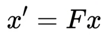
F称为状态转移矩阵,x为轨迹在t-1时刻的均值,该公式预测t时刻的x'。

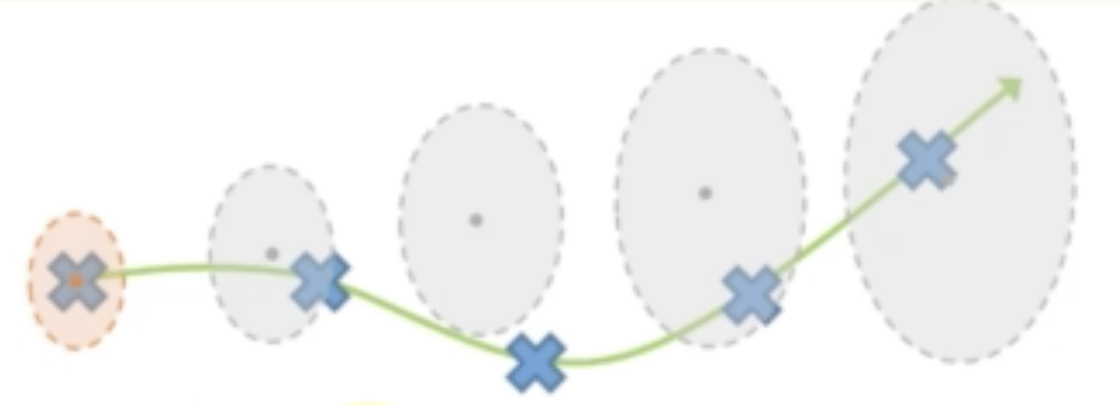
在上图中,我们可以看到,在![]() 有一个变量的协方差范围,通过状态转移矩阵
有一个变量的协方差范围,通过状态转移矩阵![]() 得到一个状态预测
得到一个状态预测![]() 的协方差。
的协方差。
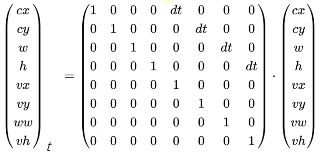
如果是横竖运动的话,那么状态转移矩阵如上图的中间部分所示,在该矩阵中,对角线全是1,与位置相关的变量有一个dt。其中状态值的cx、cy、w、h分别表示目标框的中心点坐标和目标框的宽和高。对于速度而言,由于是横竖运动,所以对角线为1。
我们通过运动模型(motion model)来进行预测。除了状态的变化,运动到新的位置的时候,协方差矩阵也会变化。由于不确定性,它的协方差矩阵可能会变得越来越大,所以我们还要进行协方差的预测。
- 协方差预测:
协方差指的是两个随机变量,当它们不满足相同分布,且有关联的时候,可以描述两者之间的相关性。具体可以参考概率论整理(二) 中的协方差及相关系数。‘
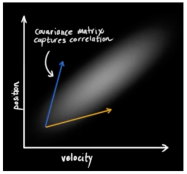
上图中的椭圆形区域就表示了位置和速度的协方差的关联性。如果知道状态转移矩阵的话,我们可以通过以下公式来求出下一时刻的协方差矩阵。
![]()
P为轨迹在t-1时刻的协方差,P'是t时刻的协方差。F是状态转移矩阵,![]() 是其转置。Q为系统的噪声矩阵,一般初始化为很小的值。
是其转置。Q为系统的噪声矩阵,一般初始化为很小的值。
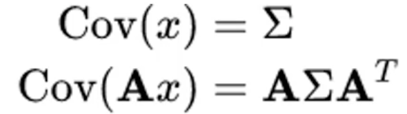
我们知道如果x的协方差是∑的话,则x左乘一个矩阵A后,那么Ax的协方差为![]() 。
。
正如上图所示,当目标运动到新的位置,那么它有新的不确定性,并且跟之前是不同的,也就是两个位置有不同的协方差。
- 更新:
基于t时刻检测到的detection,校正与其关联的轨迹(track)的状态,得到一个更精确的结果。
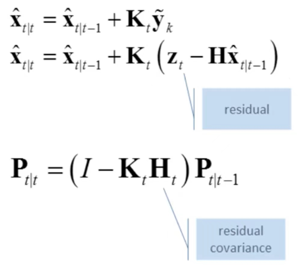
- 在上面的公式(3)中,z为detection的均值向量,不包含速度变化值,即z=[cx,cy,a,h],这里的a不是宽,而是纵横比;H称为测量矩阵,它将轨迹的均值向量x'映射到测量空间,该公式计算detection和轨迹的均值误差;y称为innovation(新息)。
- 在公式(4)中,R为检测器的噪声矩阵,它是一个4*4的对角矩阵,对角线上的值分别为中心点两个坐标以及宽高的噪声,以任意值初始化。该公式先将协方差矩阵P'映射到测量空间,然后再加上噪声矩阵R。
- 在公式(5)中,计算卡尔曼增益K,卡尔曼增益用于估计误差的重要程度。
- 在公式(6)和(7)中,得到更新后的均值向量x和协方差矩阵P。
当我们有测量值的时候,我们想用它来修正估计值。测量值是在状态空间(位置-速度空间),当我们有了measurement之后,我们需要将其映射到测量空间,测量空间是通过传感器的reading测量来得到的,所以我们需要有一个映射,这个映射就是通过测量矩阵![]() ,它就是一个模型选择矩阵(model selection matrix)。
,它就是一个模型选择矩阵(model selection matrix)。

我们可以只选择与状态相关的变量,而把它的变化值![]() 、
、![]() 不选择。
不选择。
为了获取校正值(correction),我们必须知道预测的误差,所以我们会求一个差值(residual),又称为新息(innovation)。它是通过计算预测值(predicted measurement)和观测值(obtained measurement)两者之差来获得。

上图中![]() 就是预测值,
就是预测值,![]() 为观测值。上面的式子就是状态公式,而下面的就是协方差公式。
为观测值。上面的式子就是状态公式,而下面的就是协方差公式。

另外一个问题是,我们的传感器也是有噪声的,我们假定它也是有一个正态分布的。所以它既有reading,也有random noise。在上图的右下角的图,我们即有了一个预测值(紫红色部分),还有传感器的测量值(绿色部分),它们都是正态分布的。我们想在预测值和测量值之间找到最优解。
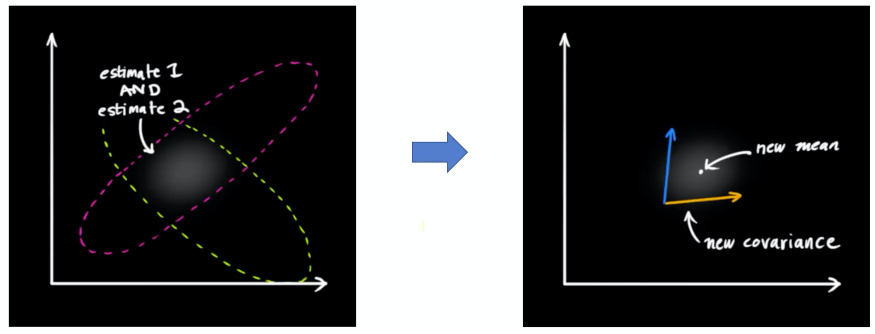
这两个分布重叠的部分就是我们认为更合理的分布。把两个具有不同均值和方差的正态分布相乘,会得到一个新的具有独立均值和方差的正态分布。也就是我们得到右图中新的分布,它有新的均值和新的方差。
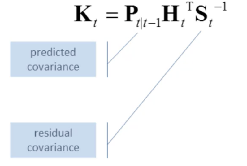
得到新的分布,我们可以推出一个卡尔曼增益(Kalman Gain),它是为了表明我们更倾向于预测值还是观测值。我们更倾向于谁,其实有一个比例,这个比例可以通过卡尔曼增益来计算出来。
有了卡尔曼增益,我们就可以更新状态和协方差矩阵了。校正以后,我们再把校正的值作为新的状态值再往前递推作为新一轮的起点,通过时间上的迭代在每一步来获取新的状态。总体流程图如下:
- 卡尔曼滤波器代码实现
import numpy as np
import scipy.linalg


"""
表中显示了N度的卡方分布的0.95分位数
自由度(包含N=1、…、9的值)
"""
chi2inv95 = {
    1: 3.8415,
    2: 5.9915,
    3: 7.8147,
    4: 9.4877,
    5: 11.070,
    6: 12.592,
    7: 14.067,
    8: 15.507,
    9: 16.919}


class KalmanFilter(object):
    """
    卡尔曼滤波器
    8维度的状态空间
        x, y, a, h, vx, vy, va, vh
    对于每一个轨迹,由一个卡尔曼滤波器预测状态分布,每个轨迹记录自己的均值和方差作为滤波器的输入
    8维状态空间,包含边界框中心点位置(x,y),纵横比a,高度h和它们各自的速度。
    物体运动遵循恒速模型,边界框位置(x,y,a,h)被视为状态空间的直接观察(线性观察模型)
    """

    def __init__(self):
        # 初始维度,dt为预测状态转移矩阵中的dt
        ndim, dt = 4, 1.

        # 构造状态转移矩阵F(8*8的矩阵,对角线为1,与位置相关的值为dt)
        self._motion_mat = np.eye(2 * ndim, 2 * ndim)
        for i in range(ndim):
            self._motion_mat[i, ndim + i] = dt
        # 构造测量矩阵H,将均值向量映射到测量空间
        self._update_mat = np.eye(ndim, 2 * ndim)

        # 依据当前状态估计(高度)选择运动和观测不确定性,这些权重控制模型中的不确定性
        self._std_weight_position = 1. / 20
        self._std_weight_velocity = 1. / 160

    def initiate(self, measurement):
        """从未关联的测量重新生成新的轨迹
        measurement: 观测值,也就是边界框的坐标值(x,y,a,h)
        返回的是一个均值向量(8维)和一个协方差矩阵(8*8)
        """
        # 中心位置
        mean_pos = measurement
        # 将初始速度初始化为0
        mean_vel = np.zeros_like(mean_pos)
        # 拼接中心位置和初始速度构建均值向量(8维)
        mean = np.r_[mean_pos, mean_vel]
        # 构建方差
        std = [
            # 对观测值进行一定的加权
            2 * self._std_weight_position * measurement[3],
            2 * self._std_weight_position * measurement[3],
            1e-2,
            2 * self._std_weight_position * measurement[3],
            10 * self._std_weight_velocity * measurement[3],
            10 * self._std_weight_velocity * measurement[3],
            1e-5,
            10 * self._std_weight_velocity * measurement[3]]
        # 构建协方差(8*8)
        covariance = np.diag(np.square(std))
        return mean, covariance

    def predict(self, mean, covariance):
        """执行卡尔曼滤波器的预测步骤
        mean: 上一步的均值向量
        covariance:上一步的协方差矩阵
        返回当前时刻的状态和协方差
        """
        # 预测的位置方差
        std_pos = [
            self._std_weight_position * mean[3],
            self._std_weight_position * mean[3],
            1e-2,
            self._std_weight_position * mean[3]]
        # 预测的速度方差
        std_vel = [
            self._std_weight_velocity * mean[3],
            self._std_weight_velocity * mean[3],
            1e-5,
            self._std_weight_velocity * mean[3]]
        # 初始化噪声矩阵Q
        motion_cov = np.diag(np.square(np.r_[std_pos, std_vel]))
        # 预测t时刻的状态
        # x'=Fx
        mean = np.dot(self._motion_mat, mean)
        # 预测t时刻的协方差
        # P'=FPF^T+Q
        covariance = np.linalg.multi_dot((
            self._motion_mat, covariance, self._motion_mat.T)) + motion_cov

        return mean, covariance

    def project(self, mean, covariance):
        """投影状态分布到测量空间
        mean: 预测出的均值向量(8维)
        covariance: 预测出的协方差(8*8)
        返回投影后的均值向量和协方差S
        """
        std = [
            self._std_weight_position * mean[3],
            self._std_weight_position * mean[3],
            1e-1,
            self._std_weight_position * mean[3]]
        # 构建噪声矩阵R
        innovation_cov = np.diag(np.square(std))
        # 将均值向量映射到测量空间,即Hx'
        mean = np.dot(self._update_mat, mean)
        # 将协方差矩阵映射到测量空间,即HP'H^T
        covariance = np.linalg.multi_dot((
            self._update_mat, covariance, self._update_mat.T))
        return mean, covariance + innovation_cov

    def update(self, mean, covariance, measurement):
        """执行卡尔曼滤波器的校正步骤,通过估计值和观测值估计最新结果
        mean: 预测出的均值向量(8维)
        covariance: 预测出的协方差(8*8)
        measurement: 观测值,也就是边界框的坐标值(x,y,a,h)
        返回校正的新的均值向量和协方差
        """
        # 将均值和协方差映射到检测空间,得到Hx'和S
        projected_mean, projected_cov = self.project(mean, covariance)
        # 矩阵分解
        chol_factor, lower = scipy.linalg.cho_factor(
            projected_cov, lower=True, check_finite=False)
        # 计算卡尔曼增益K,用于估计误差的重要程度
        # 用到了cholesky矩阵分解加快求解,这里不去求矩阵的逆,如果S矩阵很大,求逆消耗时间太长
        # 所以代码中把公式两边同时乘以S,右边的S*S的逆变成了单位矩阵,转化成AX=B的形式求解
        kalman_gain = scipy.linalg.cho_solve(
            (chol_factor, lower), np.dot(covariance, self._update_mat.T).T,
            check_finite=False).T
        # y=z-Hx'
        innovation = measurement - projected_mean
        # 更新后的均值向量x=x'+Ky
        new_mean = mean + np.dot(innovation, kalman_gain.T)
        # 更新后的协方差矩阵P=(I-KH)P'
        new_covariance = covariance - np.linalg.multi_dot((
            kalman_gain, projected_cov, kalman_gain.T))
        return new_mean, new_covariance

    def gating_distance(self, mean, covariance, measurements,
                        only_position=False):
        """计算预测值和观测值的马氏距离
        mean: 预测出的均值向量(8维)
        covariance: 预测出的协方差(8*8)
        measurements: 观测值,也就是边界框的坐标值(x,y,a,h)
        返回一个长度为N的数组,其中第i个元素包含(mean,convariance)和measurements[i]之间的
        平方马氏距离
        """
        # 将均值和协方差映射到检测空间
        mean, covariance = self.project(mean, covariance)
        if only_position:
            mean, covariance = mean[:2], covariance[:2, :2]
            measurements = measurements[:, :2]
        # 矩阵分解
        cholesky_factor = np.linalg.cholesky(covariance)
        d = measurements - mean
        z = scipy.linalg.solve_triangular(
            cholesky_factor, d.T, lower=True, check_finite=False,
            overwrite_b=True)
        # 计算平方马氏距离
        squared_maha = np.sum(z * z, axis=0)
        return squared_maha
DeepSort代码整体流程
对于整个图像的目标检测,我们使用的是YOLOV5,但我们这里不会具体再介绍YOLOV5的细节,具体可以参考YOLO系列介绍(二) 中的YOLOV5。
我们来看一下DeepSort的目标检测器
import numpy as np


class Detection(object):
    # 目标检测器

    def __init__(self, tlwh, cls_, confidence, feature):
        '''
        tlwh: 边界框(t:边界框左上角x坐标;l:边界框左上角y坐标;w:边界框宽;h:边界框高)
        confidence: 置信度
        feature: 描述图中目标的向量
        '''
        self.tlwh = np.asarray(tlwh, dtype=np.float)
        self.cls_ = cls_
        self.confidence = float(confidence)
        self.feature = np.asarray(feature, dtype=np.float32)

    def to_tlbr(self):
        """将边界框(tlwh)转化为左上角坐标和右下角坐标的格式
        """
        ret = self.tlwh.copy()
        ret[2:] += ret[:2]
        return ret

    def to_xyah(self):
        """将边界框(tlwh)转化为左上角坐标,横纵比,边界框高的格式
        """
        ret = self.tlwh.copy()
        ret[:2] += ret[2:] / 2
        ret[2] /= ret[3]
        return ret
这里我们可以看到它就是把检测边界框的值做一些后续需要的格式变换。
接下来是计算两个目标之间的最近距离的工具类
import numpy as np


def _pdist(a, b):
    """用于计算成对点之间的平方距离(欧式距离)
    a: N*M的矩阵,代表N个样本,每个样本有M个数值
    b: L*M的矩阵,代表L个样本,每个样本有M个数值
    返回N*L的矩阵,比如dist[i][j]代表a[i]和b[j]之间的平方和距离
    """
    a, b = np.asarray(a), np.asarray(b)
    if len(a) == 0 or len(b) == 0:
        return np.zeros((len(a), len(b)))
    a2, b2 = np.square(a).sum(axis=1), np.square(b).sum(axis=1)
    r2 = -2. * np.dot(a, b.T) + a2[:, None] + b2[None, :]
    r2 = np.clip(r2, 0., float(np.inf))
    return r2


def _cosine_distance(a, b, data_is_normalized=False):
    """计算成对点之间的余弦距离
    a: N*M的矩阵,代表N个样本,每个样本有M个数值
    b: L*M的矩阵,代表L个样本,每个样本有M个数值
    返回N*L的矩阵,比如dist[i][j]代表a[i]和b[j]之间的余弦距离
    """
    if not data_is_normalized:
        a = np.asarray(a) / np.linalg.norm(a, axis=1, keepdims=True)
        b = np.asarray(b) / np.linalg.norm(b, axis=1, keepdims=True)
    return 1. - np.dot(a, b.T)


def _nn_euclidean_distance(x, y):
    """ 按欧式距离来求最近邻距离矩阵
    返回对于每一个y最小的x的欧式距离
    """
    distances = _pdist(x, y)
    return np.maximum(0.0, distances.min(axis=0))


def _nn_cosine_distance(x, y):
    """ 按余弦距离来求最近邻距离矩阵
    返回对于每一个y最小的x的余弦距离
    """
    distances = _cosine_distance(x, y)
    return distances.min(axis=0)


class NearestNeighborDistanceMetric(object):
    """
    对于每个目标,返回最近距离的距离度量,即与到目前为止已观察到的任何样本的最接近距离
    """

    def __init__(self, metric, matching_threshold, budget=None):
        '''
        metric:字符串类型,要么是欧式距离要么是余弦距离
        matching_threshold: 匹配阈值,距离较大的样本对被认为是无效的匹配
        budget: 如果不是None,则将每个类别的样本最多固定为该数字,删除达到budget时最古老的样本
        '''

        if metric == "euclidean":
            self._metric = _nn_euclidean_distance
        elif metric == "cosine":
            self._metric = _nn_cosine_distance
        else:
            raise ValueError(
                "Invalid metric; must be either 'euclidean' or 'cosine'")
        self.matching_threshold = matching_threshold
        self.budget = budget
        self.samples = {}

    def partial_fit(self, features, targets, active_targets):
        """用新的数据更新测量距离
        features:N*M的矩阵,代表N个特征,每个特征有M个维度
        targets: 关联目标的整型ID
        active_targets: 当前活跃的目标的列表
        传入特征列表及其对应的ID,构造一个活跃目标的特征字典
        """
        for feature, target in zip(features, targets):
            # 对应目标下添加新的特征,更新特征集合
            # samples字典  d: feature list
            self.samples.setdefault(target, []).append(feature)
            if self.budget is not None:
                # 只考虑budget个目标,超过直接忽略
                self.samples[target] = self.samples[target][-self.budget:]
        # 筛选激活的目标
        self.samples = {k: self.samples[k] for k in active_targets}

    def distance(self, features, targets):
        """计算特征和目标之间的距离
        features:N*M的矩阵,代表N个特征,每个特征有M个维度
        targets: 和给定的特征相匹配的目标列表
        返回一个成本矩阵,元素(i,j)包含targets[i]和features[j]之间最近的距离
        """
        cost_matrix = np.zeros((len(targets), len(features)))
        for i, target in enumerate(targets):
            cost_matrix[i, :] = self._metric(self.samples[target], features)
        return cost_matrix
轨迹类
class TrackState:
    """
    单个目标轨迹状态的枚举类型
    新创建的轨迹分类为Tentative:直到收集到足够的证据为止
    然后,跟踪状态更改为Confirmed
    不再活跃的轨迹被归类为Deleted,以将其标记为从有效集中删除
    """
    Tentative = 1
    Confirmed = 2
    Deleted = 3


class Track:
    """
    具有状态空间(x,y,a,h)并关联速度的单个目标轨迹,
    其中(x,y)是边界框的中心,a是宽高比,h是高度
    """

    def __init__(self, mean, cls_, covariance, track_id, n_init, max_age,
                 feature=None):
        """
        mean:初始状态分布的均值向量
        covariance:初始状态分布的协方差矩阵
        track_id:唯一的轨迹标识符
        n_init:确认轨迹之前的连续检测次数,在第一个n_init帧中
        第一个未命中的情况下将跟踪状态设置为Deleted
        max_age:跟踪状态设置为Deleted之前的最大连续未命中数;代表一个轨迹的存活期限
        """
        self.mean = mean
        self.cls_ = cls_
        self.covariance = covariance
        self.track_id = track_id
        # 测量更新总数,代表匹配上了多少次,匹配次数超过n_init,设置Confirmed状态
        # hits每次调用update函数的时候+1
        self.hits = 1
        # 自第一次出现以来的总帧数
        self.age = 1
        # 自上次测量更新以来的总帧数,每次调用predict函数的时候+1
        self.time_since_update = 0
        # 当前轨迹状态,初始化为Tentative状态
        self.state = TrackState.Tentative
        # 特征缓存,每次测量更新时,相关特征向量添加到此列表中
        # 每个轨迹对应多个features
        self.features = []
        if feature is not None:
            self.features.append(feature)

        self._n_init = n_init
        self._max_age = max_age

    def to_tlwh(self):
        """将当前边界框的坐标转换成(左上角x,左上角y,宽,高)
        """
        ret = self.mean[:4].copy()
        ret[2] *= ret[3]
        ret[:2] -= ret[2:] / 2
        return ret

    def to_tlbr(self):
        """将当前边界框的坐标转换成(左上角x,左上角y,右下角x,右下角y)
        """
        ret = self.to_tlwh()
        ret[2:] = ret[:2] + ret[2:]
        return ret

    def predict(self, kf):
        """使用卡尔曼滤波器预测步骤将状态分布传播到当前时间步
        kf:卡尔曼滤波器对象
        """
        self.mean, self.covariance = kf.predict(self.mean, self.covariance)
        self.age += 1
        self.time_since_update += 1

    def update(self, kf, detection):
        """执行卡尔曼滤波器测量更新步骤并更新特征缓存
        kf:卡尔曼滤波器对象
        detection:所关联的边界框
        """
        self.mean, self.covariance = kf.update(
            self.mean, self.covariance, detection.to_xyah())
        self.features.append(detection.feature)
        self.cls_ = detection.cls_

        self.hits += 1
        self.time_since_update = 0
        # hits代表匹配上了多少次,匹配次数超过n_init,设置Confirmed状态
        # 连续匹配上n_init帧的时候,转变为确定态
        if self.state == TrackState.Tentative and self.hits >= self._n_init:
            self.state = TrackState.Confirmed

    def mark_missed(self):
        """将当前轨迹标记为missed(当前时间步无关联)
        """
        # 如果在处于Tentative态的情况下没有匹配上任何边界框,转变为删除态
        if self.state == TrackState.Tentative:
            self.state = TrackState.Deleted
        elif self.time_since_update > self._max_age:
            # 如果time_since_update超过max_age,设置Deleted状态
            # 即失配连续达到max_age次数时,转变为删除态
            self.state = TrackState.Deleted

    def is_tentative(self):
        """判断是否是Tentative状态
        """
        return self.state == TrackState.Tentative

    def is_confirmed(self):
        """判断是否是Confirmed状态
        """
        return self.state == TrackState.Confirmed

    def is_deleted(self):
        """判断是否是Deleted状态
        """
        return self.state == TrackState.Deleted
计算IoU的工具函数
from __future__ import absolute_import
import numpy as np
from . import linear_assignment


def iou(bbox, candidates):
    """计算交并比
    bbox: 目标边界框,格式为(左上角x,左上角y,宽,高)
    candidates: 候选框矩阵,它的每一行格式与bbox相同
    返回IoU值,如果该值较高,意味着目标较多的被候选框遮挡
    """
    # 获取目标边界框左上角坐标和右下角坐标
    bbox_tl, bbox_br = bbox[:2], bbox[:2] + bbox[2:]
    # 获取众多候选框的左上角坐标和右下角坐标
    candidates_tl = candidates[:, :2]
    candidates_br = candidates[:, :2] + candidates[:, 2:]

    tl = np.c_[np.maximum(bbox_tl[0], candidates_tl[:, 0])[:, np.newaxis],
               np.maximum(bbox_tl[1], candidates_tl[:, 1])[:, np.newaxis]]
    br = np.c_[np.minimum(bbox_br[0], candidates_br[:, 0])[:, np.newaxis],
               np.minimum(bbox_br[1], candidates_br[:, 1])[:, np.newaxis]]
    wh = np.maximum(0., br - tl)
    # 计算交集
    area_intersection = wh.prod(axis=1)
    # 获取目标边界框的面积
    area_bbox = bbox[2:].prod()
    # 获取候选框的面积
    area_candidates = candidates[:, 2:].prod(axis=1)
    # 计算IoU
    return area_intersection / (area_bbox + area_candidates - area_intersection)


def iou_cost(tracks, detections, track_indices=None,
             detection_indices=None):
    """计算轨迹和目标边界框之间的IoU距离矩阵
    tracks:轨迹的列表(包含了轨迹中所有的目标边界框)
    detections:测量目标边界框的列表
    track_indices:轨迹列表索引
    detection_indices:测量目标边界框列表索引
    返回一个成本矩阵(包含每一个轨迹和每一个目标的IoU)
    """
    if track_indices is None:
        track_indices = np.arange(len(tracks))
    if detection_indices is None:
        detection_indices = np.arange(len(detections))
    # 初始化一个全为0的成本矩阵
    cost_matrix = np.zeros((len(track_indices), len(detection_indices)))
    for row, track_idx in enumerate(track_indices):
        if tracks[track_idx].time_since_update > 1:
            cost_matrix[row, :] = linear_assignment.INFTY_COST
            continue
        # 获取轨迹中某一时刻的目标边界框
        bbox = tracks[track_idx].to_tlwh()
        # 获取所有测量目标边界框的列表
        candidates = np.asarray([detections[i].tlwh for i in detection_indices])
        # 获取该时刻轨迹的目标边界框与所有测量边界框的IoU
        cost_matrix[row, :] = 1. - iou(bbox, candidates)
    return cost_matrix
线性分配问题(通过匈牙利算法匹配轨迹与边界框)
from __future__ import absolute_import
import numpy as np
from scipy.optimize import linear_sum_assignment as linear_assignment
from . import kalman_filter


INFTY_COST = 1e+5


def min_cost_matching(
        distance_metric, max_distance, tracks, detections, track_indices=None,
        detection_indices=None):
    """使用匈牙利算法解决线性分配问题,传入门控余弦距离成本或IoU成本
    distance_metric:N*M的成本矩阵,就是轨迹和边界框之间的关联成本
    max_distance:门控阈值,大于该阈值,关联会被忽略
    tracks:当前步骤预测的轨迹列表
    detections:当前步的边界框列表
    track_indices:轨迹索引
    detection_indices:边界框索引
    返回一个元组,包含三个列表,一个是匹配的轨迹和边界框索引;一个是未匹配的轨迹索引;
    一个是未匹配的边界框索引
    """
    # 分配轨迹索引
    if track_indices is None:
        track_indices = np.arange(len(tracks))
    # 分配边界框索引
    if detection_indices is None:
        detection_indices = np.arange(len(detections))

    if len(detection_indices) == 0 or len(track_indices) == 0:
        return [], track_indices, detection_indices  # Nothing to match.
    # 计算成本矩阵
    cost_matrix = distance_metric(
        tracks, detections, track_indices, detection_indices)
    # 如果成本矩阵大于门控阈值,修改成本矩阵的值
    cost_matrix[cost_matrix > max_distance] = max_distance + 1e-5
    # 执行匈牙利算法,得到指派成功的索引对,行索引为轨迹的索引,列索引为边界框的索引
    row_indices, col_indices = linear_assignment(cost_matrix)
    # 初始化三个返回列表
    matches, unmatched_tracks, unmatched_detections = [], [], []
    # 找出未匹配的边界框
    for col, detection_idx in enumerate(detection_indices):
        if col not in col_indices:
            unmatched_detections.append(detection_idx)
    # 找出未匹配的轨迹
    for row, track_idx in enumerate(track_indices):
        if row not in row_indices:
            unmatched_tracks.append(track_idx)
    # 遍历匹配的(轨迹,边界框)索引对
    for row, col in zip(row_indices, col_indices):
        track_idx = track_indices[row]
        detection_idx = detection_indices[col]
        # 如果相应的成本矩阵中的值大于门控阈值,也视为未匹配成功
        if cost_matrix[row, col] > max_distance:
            unmatched_tracks.append(track_idx)
            unmatched_detections.append(detection_idx)
        else:  # 匹配成功
            matches.append((track_idx, detection_idx))
    return matches, unmatched_tracks, unmatched_detections


def matching_cascade(
        distance_metric, max_distance, cascade_depth, tracks, detections,
        track_indices=None, detection_indices=None):
    """执行级联匹配步骤
    distance_metric:N*M的成本矩阵,就是轨迹和边界框之间的关联成本
    max_distance:门控阈值,大于该阈值,关联会被忽略
    cascade_depth:级联深度,应设置为最大轨迹寿命
    tracks:当前步骤预测的轨迹列表
    detections:当前步的边界框列表
    track_indices:轨迹索引
    detection_indices:边界框索引
    返回一个元组,包含三个列表,一个是匹配的轨迹和边界框索引;一个是未匹配的轨迹索引;
    一个是未匹配的边界框索引
    """
    # 分配轨迹索引
    if track_indices is None:
        track_indices = list(range(len(tracks)))
    # 分配边界框索引
    if detection_indices is None:
        detection_indices = list(range(len(detections)))

    # 将所有边界框暂定为未匹配边界框
    unmatched_detections = detection_indices
    # 初始化匹配集matches M <- ø
    matches = []
    # 从小到大依次对每个深度的轨迹做匹配
    for level in range(cascade_depth):
        # 如果没有未匹配边界框,退出循环
        if len(unmatched_detections) == 0:  # No detections left
            break
        # 当前深度的所有轨迹索引
        # 步骤6:根据帧数来挑选轨迹
        track_indices_l = [
            k for k in track_indices
            if tracks[k].time_since_update == 1 + level
        ]
        # 如果当前深度没有轨迹,继续
        if len(track_indices_l) == 0:  # Nothing to match at this level
            continue
        # 步骤7:调用min_cost_matching函数进行匹配
        matches_l, _, unmatched_detections = \
            min_cost_matching(
                distance_metric, max_distance, tracks, detections,
                track_indices_l, unmatched_detections)
        # 步骤8:将匹配成功的列表添加到匹配集中
        matches += matches_l
    # 步骤9:将匹配集剔除掉,获取未匹配轨迹集
    unmatched_tracks = list(set(track_indices) - set(k for k, _ in matches))
    return matches, unmatched_tracks, unmatched_detections


def gate_cost_matrix(
        kf, cost_matrix, tracks, detections, track_indices, detection_indices,
        gated_cost=INFTY_COST, only_position=False):
    """门控成本矩阵:通过计算卡尔曼滤波的状态分布和测量值之间的距离对成本矩阵进行限制。
    成本矩阵中的距离是轨迹和边界框之间的外观相似度
    如果一个轨迹要去匹配两个外观特征非常相似的边界框,很容易出错
    分别让两个边界框计算与这个轨迹的马氏距离,并使用一个阈值gating_threshold进行限制
    就可以将马氏距离较远的那个边界框区分开,从而减少错误的匹配
    kf:卡尔曼滤波器对象
    cost_matrix:轨迹和边界框的关联成本矩阵
    tracks:当前步骤预测的轨迹列表
    detections:当前步的边界框列表
    track_indices:轨迹索引
    detection_indices:边界框索引
    gated_cost:代价矩阵中与不可行关联相对应的条目设置此值,默认是一个很大的值
    only_position:如果是Ture的话,则在门控期间仅考虑状态分布的x、y的位置,默认False,即用的四维状态空间
    返回修改过的成本矩阵
    """
    # 根据卡尔曼滤波获得状态分布,使成本矩阵中的不可行条目无效
    gating_dim = 2 if only_position else 4
    # 马氏距离通过测算检测与平均轨迹位置的距离超过多少标准差来考虑状态估计的不确定性
    # 通过从逆chi^2分布计算95%置信区间的阈值,排除可能较小的关联
    # 四维测量空间对应的马氏阈值为9.4877
    gating_threshold = kalman_filter.chi2inv95[gating_dim]
    # 转换边界框的坐标得到观测值
    measurements = np.asarray(
        [detections[i].to_xyah() for i in detection_indices])

    for row, track_idx in enumerate(track_indices):
        track = tracks[track_idx]
        # 计算状态分布和测量之间的选通距离
        gating_distance = kf.gating_distance(
            track.mean, track.covariance, measurements, only_position)
        # 得到成本矩阵,需要保证选通矩阵大于门控阈值
        cost_matrix[row, gating_distance > gating_threshold] = gated_cost
    return cost_matrix
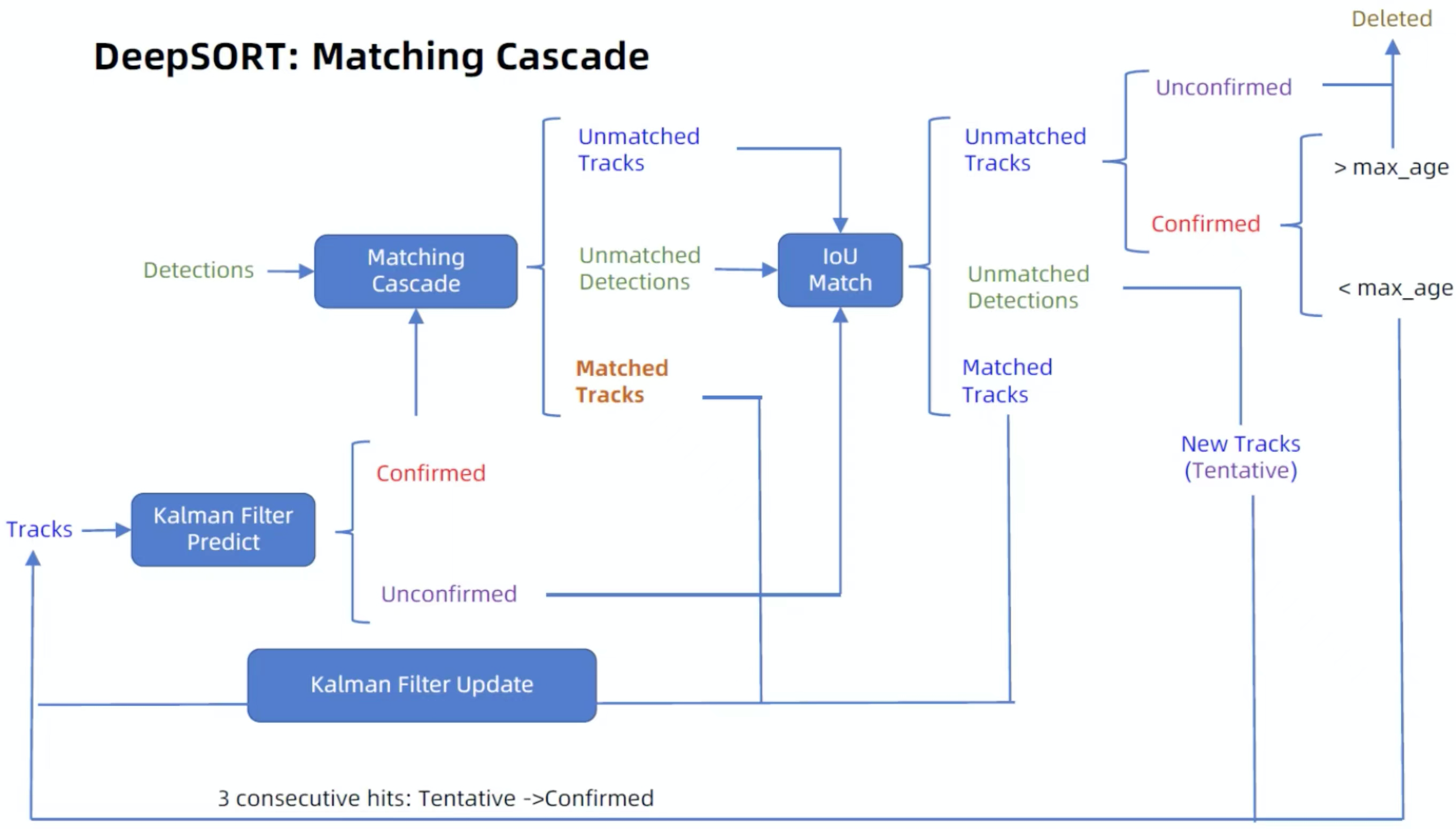
级联匹配的整体流程
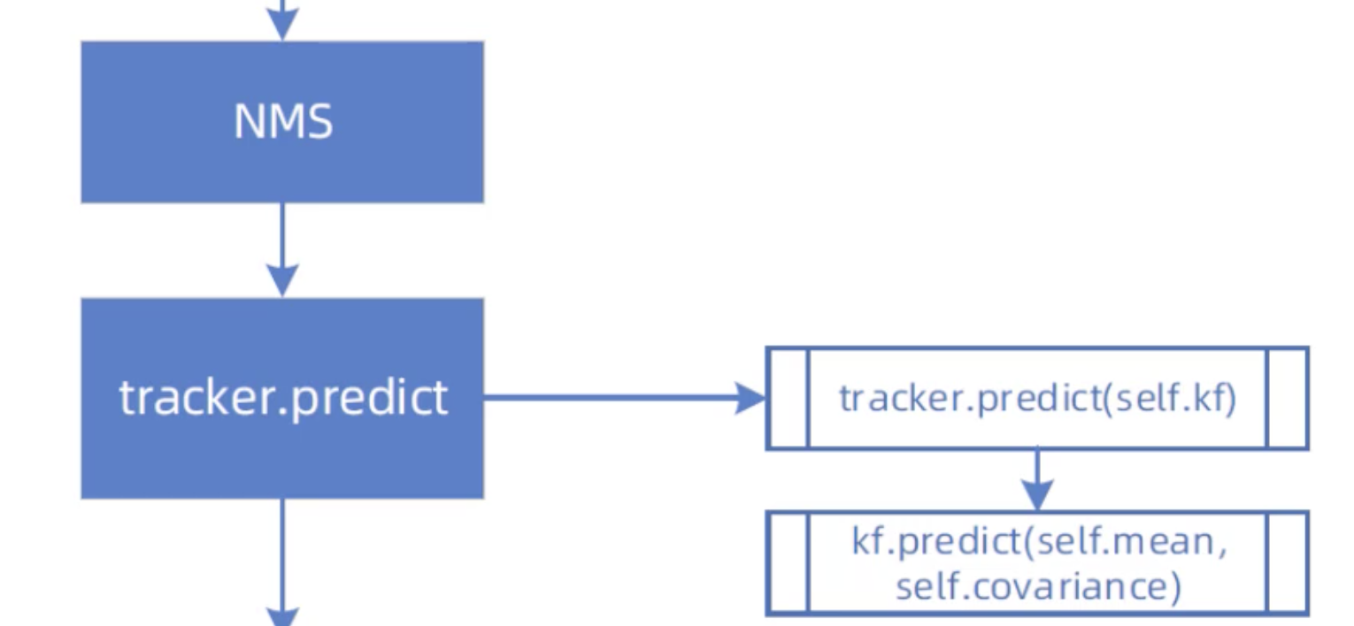
预处理(非极大值抑制),非极大值抑制是目标检测的后处理,但又是跟踪轨迹的预处理
import numpy as np


def non_max_suppression(boxes, max_bbox_overlap, scores=None):
    """非极大值抑制
    boxes:检测框列表(x, y, width, height)
    max_bbox_overlap:抑制阈值,为0.5
    scores:边界框置信度评分
    返回非极大值抑制后的边界框索引
    """
    if len(boxes) == 0:
        return []

    boxes = boxes.astype(np.float)
    pick = []
    # 获取坐标值
    x1 = boxes[:, 0]
    y1 = boxes[:, 1]
    x2 = boxes[:, 2] + boxes[:, 0]
    y2 = boxes[:, 3] + boxes[:, 1]
    # 求面积
    area = (x2 - x1 + 1) * (y2 - y1 + 1)
    if scores is not None:
        # 如果置信度评分非空,对其进行排序
        idxs = np.argsort(scores)
    else:
        idxs = np.argsort(y2)

    while len(idxs) > 0:
        # 取出置信度最小的索引,加入到列表中
        last = len(idxs) - 1
        i = idxs[last]
        pick.append(i)
        # 对于左上角的点取较大的那个
        xx1 = np.maximum(x1[i], x1[idxs[:last]])
        yy1 = np.maximum(y1[i], y1[idxs[:last]])
        # 对于右下角的点取较小的那个
        xx2 = np.minimum(x2[i], x2[idxs[:last]])
        yy2 = np.minimum(y2[i], y2[idxs[:last]])
        # 计算宽和高
        w = np.maximum(0, xx2 - xx1 + 1)
        h = np.maximum(0, yy2 - yy1 + 1)
        # 计算IoU
        overlap = (w * h) / area[idxs[:last]]
        # 比较IoU是否大于0.5,如果大于0.5则拼接,再从列表中删除
        idxs = np.delete(
            idxs, np.concatenate(
                ([last], np.where(overlap > max_bbox_overlap)[0])))

    return pick
多目标跟踪器
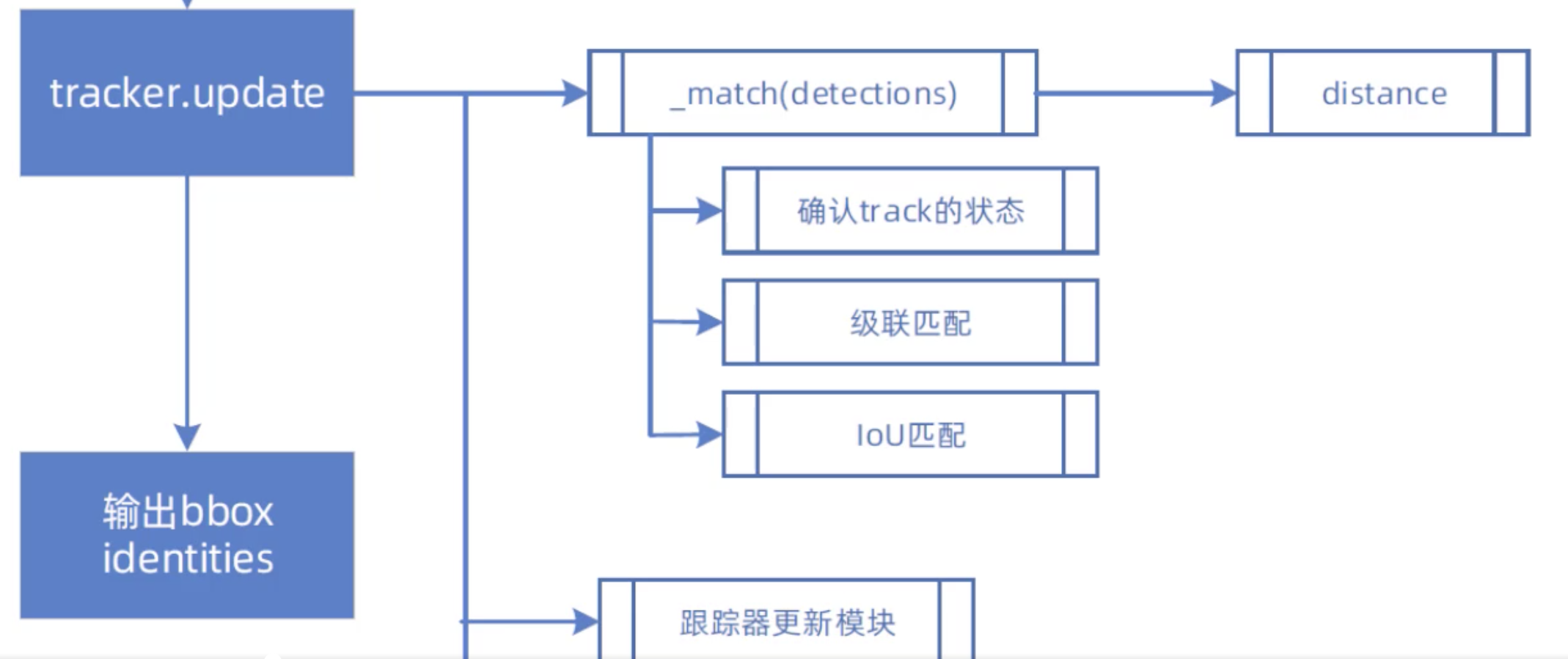
import numpy as np
from . import kalman_filter
from . import linear_assignment
from . import iou_matching
from .track import Track


class Tracker:
    """
    多目标跟踪器
    """

    def __init__(self, metric, max_iou_distance=0.7, max_age=70, n_init=3):
        """
        metric:观测(边界框)和轨迹的关联距离度量,这是一个NearestNeighborDistanceMetric对象
        max_age:轨迹关闭之前最大的未命中次数
        n_init:轨迹确认(confirmed)之前连续检测次数,默认是3,如果在前3帧中有一个未命中,
        就将轨迹设置为Deletd
        """
        self.metric = metric
        self.max_iou_distance = max_iou_distance
        self.max_age = max_age
        self.n_init = n_init
        # 卡尔曼滤波器对象
        self.kf = kalman_filter.KalmanFilter()
        # 轨迹列表
        self.tracks = []
        # 下一个分配的轨迹ID
        self._next_id = 1

    def predict(self):
        """将跟踪状态分布向前传播一步
        """
        for track in self.tracks:
            track.predict(self.kf)

    def update(self, detections):
        """执行测量跟踪和轨迹管理
        detections:当前时间步的边界框列表
        """
        # 进行级联匹配
        matches, unmatched_tracks, unmatched_detections = \
            self._match(detections)

        # 1,针对匹配上的结果
        for track_idx, detection_idx in matches:
            # 更新轨迹列表中相应的边界框
            self.tracks[track_idx].update(
                self.kf, detections[detection_idx])
        # 2,针对未匹配的轨迹,调用mark_missed进行标记
        # 轨迹失配时,若Tentative则删除,若update时间很久也删除
        for track_idx in unmatched_tracks:
            self.tracks[track_idx].mark_missed()
        # 3,针对未匹配的边界框,边界框失配,进行初始化
        for detection_idx in unmatched_detections:
            self._initiate_track(detections[detection_idx])
        # 得到最新的轨迹列表,保存的标记为Confirmed和Tentative的轨迹
        self.tracks = [t for t in self.tracks if not t.is_deleted()]

        # 获取被确认的轨迹ID
        active_targets = [t.track_id for t in self.tracks if t.is_confirmed()]
        features, targets = [], []
        for track in self.tracks:
            if not track.is_confirmed():
                continue
            # 将确认状态的轨迹的特征向量添加到features列表
            features += track.features
            # 获取每一个特征向量对应的轨迹ID
            targets += [track.track_id for _ in track.features]
            track.features = []
        # 距离度量中的特征集更新
        self.metric.partial_fit(
            np.asarray(features), np.asarray(targets), active_targets)

    def _match(self, detections):
        """轨迹与边界框匹配
        detections:当前时间步的边界框列表
        """

        def gated_metric(tracks, dets, track_indices, detection_indices):
            """门控度量
            tracks:轨迹列表
            dets:边界框列表
            track_indices:轨迹索引
            detection_indices:边界框索引
            返回门控后的成本矩阵
            """
            # 获取边界框列表的所有特征向量
            features = np.array([dets[i].feature for i in detection_indices])
            # 获取轨迹列表的所有轨迹ID
            targets = np.array([tracks[i].track_id for i in track_indices])
            # 通过最近邻(余弦距离)计算出成本矩阵(代价矩阵)
            cost_matrix = self.metric.distance(features, targets)
            # 计算门控后的成本矩阵(代价矩阵)
            cost_matrix = linear_assignment.gate_cost_matrix(
                self.kf, cost_matrix, tracks, dets, track_indices,
                detection_indices)

            return cost_matrix

        # 区分开确认状态的轨迹和未确认状态的轨迹
        confirmed_tracks = [
            i for i, t in enumerate(self.tracks) if t.is_confirmed()]
        unconfirmed_tracks = [
            i for i, t in enumerate(self.tracks) if not t.is_confirmed()]

        # 对确定状态的轨迹进行级联匹配,得到匹配的轨迹列表、不匹配的轨迹列表哦、不匹配的边界框列表
        # 传入门控后的成本矩阵
        matches_a, unmatched_tracks_a, unmatched_detections = \
            linear_assignment.matching_cascade(
                gated_metric, self.metric.matching_threshold, self.max_age,
                self.tracks, detections, confirmed_tracks)

        # 将未确定状态的轨迹和刚刚没有匹配上的轨迹组合为iou_track_candidates
        # 并进行基于IoU的匹配
        iou_track_candidates = unconfirmed_tracks + [
            k for k in unmatched_tracks_a if
            # 刚刚没有匹配上的轨迹
            self.tracks[k].time_since_update == 1]
        unmatched_tracks_a = [
            k for k in unmatched_tracks_a if
            # 并非刚刚没有匹配上的轨迹
            self.tracks[k].time_since_update != 1]
        # 对级联匹配中还没有匹配成功的目标再进行IoU匹配
        # min_cost_matching使用匈牙利算法解决线性分配问题
        # 传入iou_cost,尝试关联剩余的轨迹与未确认的轨迹
        matches_b, unmatched_tracks_b, unmatched_detections = \
            linear_assignment.min_cost_matching(
                iou_matching.iou_cost, self.max_iou_distance, self.tracks,
                detections, iou_track_candidates, unmatched_detections)
        # 组合两部分匹配
        matches = matches_a + matches_b
        unmatched_tracks = list(set(unmatched_tracks_a + unmatched_tracks_b))
        return matches, unmatched_tracks, unmatched_detections

    def _initiate_track(self, detection):
        """未匹配上的边界框进行初始化
        detection:未匹配上的边界框
        """
        # 通过卡尔曼滤波器初始化得到均值向量和协方差
        mean, covariance = self.kf.initiate(detection.to_xyah())
        # 构建轨迹对象,并添加到轨迹列表中
        self.tracks.append(Track(
            mean, detection.cls_, covariance, self._next_id, self.n_init, self.max_age,
            detection.feature))
        # 更新下一个分配的轨迹ID
        self._next_id += 1
卷积神经网络
import torch
import torch.nn as nn
import torch.nn.functional as F

class BasicBlock(nn.Module):
    """
    ResBlock
    """
    def __init__(self, c_in, c_out, is_downsample=False):
        super(BasicBlock, self).__init__()
        # 是否进行降采样,默认False
        self.is_downsample = is_downsample
        if is_downsample:
            self.conv1 = nn.Conv2d(c_in, c_out, 3, stride=2, padding=1, bias=False)
        else:
            # 第一层卷积,卷积核大小3*3
            self.conv1 = nn.Conv2d(c_in, c_out, 3, stride=1, padding=1, bias=False)
        self.bn1 = nn.BatchNorm2d(c_out)
        self.relu = nn.ReLU(True)
        # 第二层卷积,卷积核大小3*3
        self.conv2 = nn.Conv2d(c_out, c_out, 3, stride=1, padding=1, bias=False)
        self.bn2 = nn.BatchNorm2d(c_out)
        if is_downsample:
            # 如果进行降采样,使用1*1的卷积核进行降采样
            self.downsample = nn.Sequential(
                nn.Conv2d(c_in, c_out, 1, stride=2, bias=False),
                nn.BatchNorm2d(c_out)
            )
        elif c_in != c_out:  # 如果输入通道数不等于输出
            # 进行1*1卷积
            self.downsample = nn.Sequential(
                nn.Conv2d(c_in, c_out, 1, stride=1, bias=False),
                nn.BatchNorm2d(c_out)
            )
            self.is_downsample = True

    def forward(self, x):
        y = self.conv1(x)
        y = self.bn1(y)
        y = self.relu(y)
        y = self.conv2(y)
        y = self.bn2(y)
        if self.is_downsample:
            x = self.downsample(x)
        return F.relu(x.add(y), True)

def make_layers(c_in, c_out, repeat_times, is_downsample=False):
    blocks = []
    for i in range(repeat_times):
        if i == 0:
            blocks += [BasicBlock(c_in, c_out, is_downsample=is_downsample), ]
        else:
            blocks += [BasicBlock(c_out, c_out), ]
    return nn.Sequential(*blocks)

class Net(nn.Module):
    """
    主网络
    """
    def __init__(self, num_classes=751, reid=False):
        super(Net, self).__init__()
        # 将宽128,高64,3通道图片送入网络
        # 输出64*32*64
        self.conv = nn.Sequential(
            nn.Conv2d(3, 64, 3, stride=1, padding=1),
            nn.BatchNorm2d(64),
            nn.ReLU(inplace=True),
            # nn.Conv2d(32,32,3,stride=1,padding=1),
            # nn.BatchNorm2d(32),
            # nn.ReLU(inplace=True),
            nn.MaxPool2d(3, 2, padding=1),
        )
        # 输出64*32*64
        self.layer1 = make_layers(64, 64, 2, False)
        # 输出32*16*128
        self.layer2 = make_layers(64, 128, 2, True)
        # 输出16*8*256
        self.layer3 = make_layers(128, 256, 2, True)
        # 输出8*4*512
        self.layer4 = make_layers(256, 512, 2, True)
        # 输出1*1*512
        self.avgpool = nn.AvgPool2d((8, 4), 1)
        self.reid = reid
        # 分类器,751种分类
        self.classifier = nn.Sequential(
            nn.Linear(512, 256),
            nn.BatchNorm1d(256),
            nn.ReLU(inplace=True),
            nn.Dropout(),
            nn.Linear(256, num_classes),
        )

    def forward(self, x):
        x = self.conv(x)
        x = self.layer1(x)
        x = self.layer2(x)
        x = self.layer3(x)
        x = self.layer4(x)
        x = self.avgpool(x)
        x = x.view(x.size(0), -1)
        # B x 128
        if self.reid:
            x = x.div(x.norm(p=2, dim=1, keepdim=True))
            return x
        # classifier
        x = self.classifier(x)
        return x


if __name__ == '__main__':
    net = Net()
    x = torch.randn(4, 3, 128, 64)
    y = net(x)
    print(y)
    print(y.size())
运行结果
tensor([[ 0.5376, -0.1476, -0.6526,  ...,  0.3392, -0.3412, -0.3442],
        [ 0.4959, -0.4458, -1.0641,  ...,  0.2254, -0.0602,  0.4078],
        [ 0.3850, -0.1913, -1.0202,  ...,  0.0398,  0.3249,  0.0951],
        [ 0.2672, -0.3080,  0.5000,  ...,  0.8824,  0.2869,  0.9582]],
       grad_fn=<AddmmBackward>)
torch.Size([4, 751])
特征提取器
import torch
import torchvision.transforms as transforms
import numpy as np
import cv2
import logging

from .model import Net

class Extractor(object):
    """
    特征提取器
    """
    def __init__(self, model_path, use_cuda=True):
        # 初始化卷积神经网络
        self.net = Net(reid=True)
        self.device = "cuda" if torch.cuda.is_available() and use_cuda else "cpu"
        # 导入模型参数
        state_dict = torch.load(model_path, map_location=lambda storage, loc: storage)['net_dict']
        self.net.load_state_dict(state_dict)
        logger = logging.getLogger("root.tracker")
        logger.info("Loading weights from {}... Done!".format(model_path))
        self.net.to(self.device)
        self.size = (64, 128)
        self.norm = transforms.Compose([
            # 归一化,转成tensor
            transforms.ToTensor(),
            # 标准化,第一个元组表示各个通道(r,g,b)的均值,第二个元组表示各个通道(r,g,b)的方差
            transforms.Normalize([0.485, 0.456, 0.406], [0.229, 0.224, 0.225]),
        ])


    def _preprocess(self, im_crops):
        """
        预处理
        im_crops:批量图片
        """
        def _resize(im, size):
            """
            修改单张图片尺寸
            """
            return cv2.resize(im.astype(np.float32) / 255., size)

        # 对批量图片的每一张图片进行修改尺寸,再恢复成批量
        im_batch = torch.cat([self.norm(_resize(im, self.size)).unsqueeze(0) for im in im_crops], dim=0).float()
        return im_batch


    def __call__(self, im_crops):
        # 对批量图像进行预处理,转成64*128大小
        im_batch = self._preprocess(im_crops)
        with torch.no_grad():
            im_batch = im_batch.to(self.device)
            # 前向运算,获取特征向量
            features = self.net(im_batch)
        return features.cpu().numpy()


if __name__ == '__main__':
    img = cv2.imread("train.jpg")[:, :, (2, 1, 0)]
    extr = Extractor("checkpoint/ckpt.t7")
    img_batch = np.expand_dims(img, axis=0)
    feature = extr(img_batch)
    print(feature.shape)
运行结果
(1, 512)
DeepSort流程
import numpy as np
import torch

from .deep.feature_extractor import Extractor
from .sort.nn_matching import NearestNeighborDistanceMetric
from .sort.detection import Detection
from .sort.tracker import Tracker

# 提供了暴露接口的白名单
__all__ = ['DeepSort']


class DeepSort(object):
    def __init__(self, model_path, max_dist=0.2, min_confidence=0.3, nms_max_overlap=1.0, max_iou_distance=0.7, max_age=70, n_init=3, nn_budget=100, use_cuda=True):
        # 检测结果置信度阈值
        self.min_confidence = min_confidence
        # 非极大抑制阈值,设置为1表示不进行抑制
        self.nms_max_overlap = nms_max_overlap
        # 用于提取一个batch图片中对应的特征
        self.extractor = Extractor(model_path, use_cuda=use_cuda)
        # 最大余弦距离,用于级联匹配,如果大于该阈值,则忽略
        max_cosine_distance = max_dist
        # 每个类别gallery最多的外观描述子的个数,如果超过,删除旧的
        nn_budget = 100
        # 最近邻距离度量
        # 对于每个目标,返回到目前为止已观察到的任何样本的最近距离(欧式或余弦)
        # 第一个参数可选cosine或euclidean
        metric = NearestNeighborDistanceMetric(
            "cosine", max_cosine_distance, nn_budget)
        # 由距离度量方法构造一个多目标追踪器
        self.tracker = Tracker(
            metric, max_iou_distance=max_iou_distance, max_age=max_age, n_init=n_init)

    def update(self, bbox_xywh, confidences, clss, ori_img):
        # 获取原图的高宽
        self.height, self.width = ori_img.shape[:2]
        # 从原图中抠取bbox对应图片并计算得到相应的特征
        features = self._get_features(bbox_xywh, ori_img)
        # 转换坐标格式
        bbox_tlwh = self._xywh_to_tlwh(bbox_xywh)
        # 筛选掉小于min_confidence的目标,并构造一个Detection对象构成的列表
        detections = [Detection(bbox_tlwh[i], clss[i], conf, features[i]) for i, conf in enumerate(
            confidences) if conf > self.min_confidence]
        # 将跟踪状态分布向前传播一步
        self.tracker.predict()
        # 执行测量更新和跟踪管理
        self.tracker.update(detections)

        # 初始化输出列表
        outputs = []
        # 对多目标追踪器的轨迹列表进行迭代
        for track in self.tracker.tracks:
            # 轨迹必须为已确认的或者未进行过一次以上的测量更新
            if not track.is_confirmed() or track.time_since_update > 1:
                continue
            # 转换轨迹坐标
            box = track.to_tlwh()
            # 转换坐标格式
            x1, y1, x2, y2 = self._tlwh_to_xyxy(box)
            # 输出列表添加坐标、轨迹分类、轨迹ID的元组
            outputs.append((x1, y1, x2, y2, track.cls_, track.track_id))
        return outputs

    @staticmethod
    def _xywh_to_tlwh(bbox_xywh):
        """
        转换中心点坐标、宽、高格式为左上角坐标、宽、高格式
        """
        if isinstance(bbox_xywh, np.ndarray):
            bbox_tlwh = bbox_xywh.copy()
        elif isinstance(bbox_xywh, torch.Tensor):
            bbox_tlwh = bbox_xywh.clone()
        bbox_tlwh[:, 0] = bbox_xywh[:, 0] - bbox_xywh[:, 2] / 2.
        bbox_tlwh[:, 1] = bbox_xywh[:, 1] - bbox_xywh[:, 3] / 2.
        return bbox_tlwh

    def _xywh_to_xyxy(self, bbox_xywh):
        """
        转换中心点坐标、宽、高格式为左上角坐标、右下角坐标格式
        """
        x, y, w, h = bbox_xywh
        x1 = max(int(x - w / 2), 0)
        x2 = min(int(x + w / 2), self.width - 1)
        y1 = max(int(y - h / 2), 0)
        y2 = min(int(y + h / 2), self.height - 1)
        return x1, y1, x2, y2

    def _tlwh_to_xyxy(self, bbox_tlwh):
        """
        转换左上角坐标、宽、高格式为左上角坐标、右下角坐标格式
        """
        x, y, w, h = bbox_tlwh
        x1 = max(int(x), 0)
        x2 = min(int(x + w), self.width - 1)
        y1 = max(int(y), 0)
        y2 = min(int(y + h), self.height - 1)
        return x1, y1, x2, y2

    def _xyxy_to_tlwh(self, bbox_xyxy):
        """
        转换左上角坐标、右下角坐标格式为左上角坐标、宽、高格式
        """
        x1, y1, x2, y2 = bbox_xyxy

        t = x1
        l = y1
        w = int(x2 - x1)
        h = int(y2 - y1)
        return t, l, w, h

    def _get_features(self, bbox_xywh, ori_img):
        """
        获取抠图部分的特征
        """
        im_crops = []
        for box in bbox_xywh:
            x1, y1, x2, y2 = self._xywh_to_xyxy(box)
            # 抠图部分
            im = ori_img[y1:y2, x1:x2]
            im_crops.append(im)
        if im_crops:
            # 对抠图部分提取特征
            features = self.extractor(im_crops)
        else:
            features = np.array([])
        return features
流程图
之前我们都是假设目标框已经选取出来了,现在我们来看一下真正跟YOLOV5的关联。
from tracker import update_tracker
import cv2


class baseDet(object):
    """
    视频检测的基础类
    """

    def __init__(self):
        # 图片尺寸
        self.img_size = 640
        # 检测置信度阈值
        self.threshold = 0.3
        self.stride = 1

    def build_config(self):

        self.faceTracker = {}
        self.faceClasses = {}
        self.faceLocation1 = {}
        self.faceLocation2 = {}
        self.frameCounter = 0
        self.currentCarID = 0
        self.recorded = []

        self.font = cv2.FONT_HERSHEY_SIMPLEX

    def feedCap(self, im):
        """
        导入视频
        """
        # 检测字典
        retDict = {
            'frame': None,
            'faces': None,
            'list_of_ids': None,
            'face_bboxes': []
        }
        # 帧数加1
        self.frameCounter += 1
        # 提取图形、目标和目标框
        im, faces, face_bboxes = update_tracker(self, im)
        # 将其添加到字典
        retDict['frame'] = im
        retDict['faces'] = faces
        retDict['face_bboxes'] = face_bboxes

        return retDict

    def init_model(self):
        raise EOFError("Undefined model type.")

    def preprocess(self):
        raise EOFError("Undefined model type.")

    def detect(self):
        raise EOFError("Undefined model type.")
YOLOV5子类
import torch
import numpy as np
from models.experimental import attempt_load
from utils.general import non_max_suppression, scale_coords
from utils.BaseDetector import baseDet
from utils.torch_utils import select_device
from utils.datasets import letterbox

class Detector(baseDet):
    """
    YOLOV5检测器的封装
    """

    def __init__(self):
        super(Detector, self).__init__()
        self.init_model()
        self.build_config()

    def init_model(self):
        # 获取模型参数
        self.weights = 'weights/yolov5s.pt'
        self.device = '0' if torch.cuda.is_available() else 'cpu'
        self.device = select_device(self.device)
        # 加载参数权重,构造YOLOV5模型实例
        model = attempt_load(self.weights, map_location=self.device)
        model.to(self.device).eval()
        model.half()
        # torch.save(model, 'test.pt')
        self.m = model
        # 获取模型的标签名称
        self.names = model.module.names if hasattr(
            model, 'module') else model.names

    def preprocess(self, img):
        """
        预处理
        返回原始图像和预处理后的图像
        """
        img0 = img.copy()
        # 根据大小调整图像
        img = letterbox(img, new_shape=self.img_size)[0]
        # 将图像调整成pytorch格式
        img = img[:, :, ::-1].transpose(2, 0, 1)
        img = np.ascontiguousarray(img)
        img = torch.from_numpy(img).to(self.device)
        img = img.half()  # 半精度
        # img = img.float()
        img /= 255.0  # 图像归一化
        if img.ndimension() == 3:
            img = img.unsqueeze(0)

        return img0, img

    def detect(self, im):
        """
        检测目标框
        """
        # 预处理
        im0, img = self.preprocess(im)
        # 将预处理后的图像传入模型,进行前向运算,获得预测边框
        pred = self.m(img, augment=False)[0]
        pred = pred.float()
        # 非极大值抑制
        pred = non_max_suppression(pred, self.threshold, 0.4)

        pred_boxes = []
        for det in pred:

            if det is not None and len(det):
                # 将检测区域缩放回原始图像大小
                det[:, :4] = scale_coords(
                    img.shape[2:], det[:, :4], im0.shape).round()

                for *x, conf, cls_id in det:
                    # 获取检测类别
                    lbl = self.names[int(cls_id)]
                    # 这里只检测人、汽车、卡车
                    if not lbl in ['person', 'car', 'truck']:
                        continue
                    # 获取坐标
                    x1, y1 = int(x[0]), int(x[1])
                    x2, y2 = int(x[2]), int(x[3])
                    # 获取坐标、类别和置信度,添加进列表
                    pred_boxes.append(
                        (x1, y1, x2, y2, lbl, conf))

        return im, pred_boxes
在baseDet中有一段
# 提取图形、目标和目标框
im, faces, face_bboxes = update_tracker(self, im)
我们来看一下它的实现,首先是deep_sort的配置文件deep_sort.yaml
DEEPSORT:
#  网络模型参数地址
  REID_CKPT: "deep_sort/deep_sort/deep/checkpoint/ckpt.t7"
  MAX_DIST: 0.2
#  最小置信度
  MIN_CONFIDENCE: 0.3
#  非极大值抑制阈值
  NMS_MAX_OVERLAP: 0.5
#  最大IoU距离
  MAX_IOU_DISTANCE: 0.7
#  跟踪状态设置为Deleted之前的最大连续未命中数;代表一个轨迹的存活期限
  MAX_AGE: 70
#  确认轨迹之前的连续检测次数
  N_INIT: 3
#  每个类别gallery最多的外观描述子的个数,如果超过,删除旧的
  NN_BUDGET: 100
from deep_sort.utils.parser import get_config
from deep_sort.deep_sort import DeepSort
import torch
import cv2

palette = (2 ** 11 - 1, 2 ** 15 - 1, 2 ** 20 - 1)
cfg = get_config()
cfg.merge_from_file("deep_sort/configs/deep_sort.yaml")
deepsort = DeepSort(cfg.DEEPSORT.REID_CKPT,
                    max_dist=cfg.DEEPSORT.MAX_DIST, min_confidence=cfg.DEEPSORT.MIN_CONFIDENCE,
                    nms_max_overlap=cfg.DEEPSORT.NMS_MAX_OVERLAP, max_iou_distance=cfg.DEEPSORT.MAX_IOU_DISTANCE,
                    max_age=cfg.DEEPSORT.MAX_AGE, n_init=cfg.DEEPSORT.N_INIT, nn_budget=cfg.DEEPSORT.NN_BUDGET,
                    use_cuda=True)


def plot_bboxes(image, bboxes, line_thickness=None):
    # Plots one bounding box on image img
    tl = line_thickness or round(
        0.002 * (image.shape[0] + image.shape[1]) / 2) + 1  # line/font thickness
    for (x1, y1, x2, y2, cls_id, pos_id) in bboxes:
        if cls_id in ['person']:
            color = (0, 0, 255)
        else:
            color = (0, 255, 0)
        c1, c2 = (x1, y1), (x2, y2)
        cv2.rectangle(image, c1, c2, color, thickness=tl, lineType=cv2.LINE_AA)
        tf = max(tl - 1, 1)  # font thickness
        t_size = cv2.getTextSize(cls_id, 0, fontScale=tl / 3, thickness=tf)[0]
        c2 = c1[0] + t_size[0], c1[1] - t_size[1] - 3
        cv2.rectangle(image, c1, c2, color, -1, cv2.LINE_AA)  # filled
        cv2.putText(image, '{} ID-{}'.format(cls_id, pos_id), (c1[0], c1[1] - 2), 0, tl / 3,
                    [225, 255, 255], thickness=tf, lineType=cv2.LINE_AA)

    return image


def update_tracker(target_detector, image):
    new_faces = []
    # 使用YOLOV5检测器对图像进行检测,得到目标框
    _, bboxes = target_detector.detect(image)
    # 坐标列表
    bbox_xywh = []
    # 置信度列表
    confs = []
    # 分类列表
    clss = []
    # 对每一个目标框做迭代
    for x1, y1, x2, y2, cls_id, conf in bboxes:
        # 获取目标框坐标值
        obj = [
            int((x1 + x2) / 2), int((y1 + y2) / 2),
            x2 - x1, y2 - y1
        ]
        # 将这些值存入列表
        bbox_xywh.append(obj)
        confs.append(conf)
        clss.append(cls_id)

    xywhs = torch.Tensor(bbox_xywh)
    confss = torch.Tensor(confs)
    # 将检测出的目标框传送到deepsort中
    # 获取坐标,轨迹分类,轨迹ID
    outputs = deepsort.update(xywhs, confss, clss, image)
    # 需要绘制的列表
    bboxes2draw = []
    # 坐标列表
    face_bboxes = []
    # 当前轨迹id列表
    current_ids = []
    for value in list(outputs):
        x1, y1, x2, y2, cls_, track_id = value
        # 绘制列表添加
        bboxes2draw.append(
            (x1, y1, x2, y2, cls_, track_id)
        )
        # 当前轨迹id列表添加
        current_ids.append(track_id)
        if cls_ == 'person':
            # 如果当前轨迹id不在历史轨迹中,则添加新的目标
            if not track_id in target_detector.faceTracker:
                target_detector.faceTracker[track_id] = 0
                face = image[y1:y2, x1:x2]
                new_faces.append((face, track_id))
            # 坐标列表添加
            face_bboxes.append(
                (x1, y1, x2, y2, cls_, track_id)
            )
    # 需要清除的轨迹id列表
    ids2delete = []
    for history_id in target_detector.faceTracker:
        if not history_id in current_ids:
            # 如果历史轨迹id不在当前轨迹id中,则将该id值-1
            target_detector.faceTracker[history_id] -= 1
        if target_detector.faceTracker[history_id] < -5:
            # 如果该id值小于-5,则放入需要清除的轨迹id列表中
            ids2delete.append(history_id)

    for ids in ids2delete:
        # 清除需要清除的轨迹id
        target_detector.faceTracker.pop(ids)
        print('-[INFO] Delete track id:', ids)
    # 在图像中进行绘制
    image = plot_bboxes(image, bboxes2draw)

    return image, new_faces, face_bboxes
撞线统计人数
import numpy as np
from tracker import update_tracker
from AIDetector_pytorch import Detector
import cv2

if __name__ == '__main__':

    video_path = '/home/jingzhi/001.avi'

    # 根据视频尺寸,填充供撞线计算使用的多边形
    width = 1920
    height = 1080
    mask_image_temp = np.zeros((height, width), dtype=np.uint8)
    # 填充第一个撞线多边形(蓝色)
    list_pts_blue = [[204, 305], [227, 431], [605, 522], [1101, 464], [1900, 601], [1902, 495],
                     [299, 375], [267, 289]]
    ndarray_pts_blue = np.array(list_pts_blue, np.int32)
    polygon_blue_value_1 = cv2.fillPoly(mask_image_temp, [ndarray_pts_blue], color=1)
    polygon_blue_value_1 = polygon_blue_value_1[:, :, np.newaxis]

    mask_image_temp = np.zeros((height, width), dtype=np.uint8)
    # 填充第二个撞线多边形(黄色)
    list_pts_yellow = [[181, 305], [207, 442], [603, 544], [1107, 485], [1898, 625], [1893, 701],
                       [594, 637], [118, 483], [109, 303]]
    ndarray_pts_yellow = np.array(list_pts_yellow, np.int32)
    polygon_yellow_value_2 = cv2.fillPoly(mask_image_temp, [ndarray_pts_yellow], color=2)
    polygon_yellow_value_2 = polygon_yellow_value_2[:, :, np.newaxis]
    # 撞线检测用的mask,包含2个多边形,(值范围0,1,2),供撞线计算使用
    polygon_mask_blue_and_yellow = polygon_blue_value_1 + polygon_yellow_value_2
    # 缩小尺寸
    polygon_mask_blue_and_yellow = cv2.resize(polygon_mask_blue_and_yellow, (width // 2, height // 2))
    # 蓝 色盘 b,g,r
    blue_color_plate = [255, 0, 0]
    # 蓝 多边形图片
    blue_image = np.array(polygon_blue_value_1 * blue_color_plate, np.uint8)
    # 黄 色盘
    yellow_color_plate = [0, 255, 255]
    # 黄 多边形图片
    yellow_image = np.array(polygon_yellow_value_2 * yellow_color_plate, np.uint8)
    # 彩色图片(值范围 0-255)
    color_polygons_images = blue_image + yellow_image
    # 缩小尺寸
    color_polygons_images = cv2.resize(color_polygons_images, (width // 2, height // 2))
    # 列表,与蓝色多边形重叠
    list_overlapping_blue_polygon = []
    # 列表,与黄色多边形重叠
    list_overlapping_yellow_polygon = []
    # 下行数量
    down_count = 0
    # 上行数量
    up_count = 0

    font_draw_number = cv2.FONT_HERSHEY_SIMPLEX
    draw_text_postion = (int((width / 2) * 0.01), int((height / 2) * 0.05))
    # 实例化YOLOV5检测器
    detector = Detector()
    # 打开视频
    capture = cv2.VideoCapture(video_path)
    fps = int(capture.get(5))
    videoWriter = None
    while True:
        # 读取每帧图片
        _, im = capture.read()
        if im is None:
            break
        # 缩小尺寸
        im = cv2.resize(im, (width // 2, height // 2))
        list_bboxs = []
        # 更新跟踪器
        output_image_frame, _, list_bboxs = update_tracker(detector, im)
        # 输出图片
        output_image_frame = cv2.add(output_image_frame, color_polygons_images)
        if len(list_bboxs) > 0:
            # 判断撞线
            for item_bbox in list_bboxs:
                x1, y1, x2, y2, _, track_id = item_bbox
                # 撞线检测点,(x1,y1),y方向偏移比例0.0-1.0
                y1_offset = int(y1 + ((y2 - y1) * 0.6))
                # 撞线的点
                y = y1_offset
                x = x1
                if polygon_mask_blue_and_yellow[y, x] == 1:
                    # 如果撞蓝多边形
                    if track_id not in list_overlapping_blue_polygon:
                        list_overlapping_blue_polygon.append(track_id)
                    # 判断黄多边形列表里是否有此轨迹id
                    if track_id in list_overlapping_yellow_polygon:
                        # 上行+1
                        up_count += 1
                        print('up count:', up_count, ', up id:', list_overlapping_yellow_polygon)
                        # 删除黄多边形列表中的此轨迹id
                        list_overlapping_yellow_polygon.remove(track_id)
                if polygon_mask_blue_and_yellow[y, x] == 2:
                    # 如果撞黄多边形
                    if track_id not in list_overlapping_yellow_polygon:
                        list_overlapping_yellow_polygon.append(track_id)
                    # 判断蓝多边形列表里是否有此轨迹id
                    if track_id in list_overlapping_blue_polygon:
                        # 下行+1
                        down_count += 1
                        print('down count:', down_count, ', down id:', list_overlapping_blue_polygon)
                        # 删除蓝多边形列表中的此轨迹id
                        list_overlapping_blue_polygon.remove(track_id)
        # 清除无用id
        list_overlapping_all = list_overlapping_yellow_polygon + list_overlapping_blue_polygon
        for id1 in list_overlapping_all:
            is_found = False
            for _, _, _, _, _, bbox_id in list_bboxs:
                if bbox_id == id1:
                    is_found = True
            if not is_found:
                # 如果没有找到,删除id
                if id1 in list_overlapping_yellow_polygon:
                    list_overlapping_yellow_polygon.remove(id1)
                if id1 in list_overlapping_blue_polygon:
                    list_overlapping_blue_polygon.remove(id1)
            # list_overlapping_blue_polygon.clear()
            # list_overlapping_yellow_polygon.clear()
        # 输出计数信息
        if videoWriter is None:
            fourcc = cv2.VideoWriter_fourcc(
                'm', 'p', '4', 'v')  # opencv3.0
            videoWriter = cv2.VideoWriter(
                'result.mp4', fourcc, fps, (im.shape[1], im.shape[0]))
        text_draw = 'DOWN: ' + str(down_count) + ', UP: ' + str(up_count)
        output_image_frame = cv2.putText(img=output_image_frame, text=text_draw,
                                         org=draw_text_postion, fontFace=font_draw_number,
                                         fontScale=0.75, color=(0, 0, 255), thickness=2)
        videoWriter.write(output_image_frame)
        cv2.imshow('Counting Demo', output_image_frame)
        cv2.waitKey(1)
    capture.release()
    cv2.destroyAllWindows()