活动地址:CSDN21天学习挑战赛
前言
本周的任务有3个,预测股票,识别验证码,识别眼睛状态。因为任务不同,那么可能会使用到不同的预处理、网络等等。
本节主要学习股票预测。
一、拆解任务
首先需要了解这次需要处理的任务,这里贴一张老师的数据展示图。
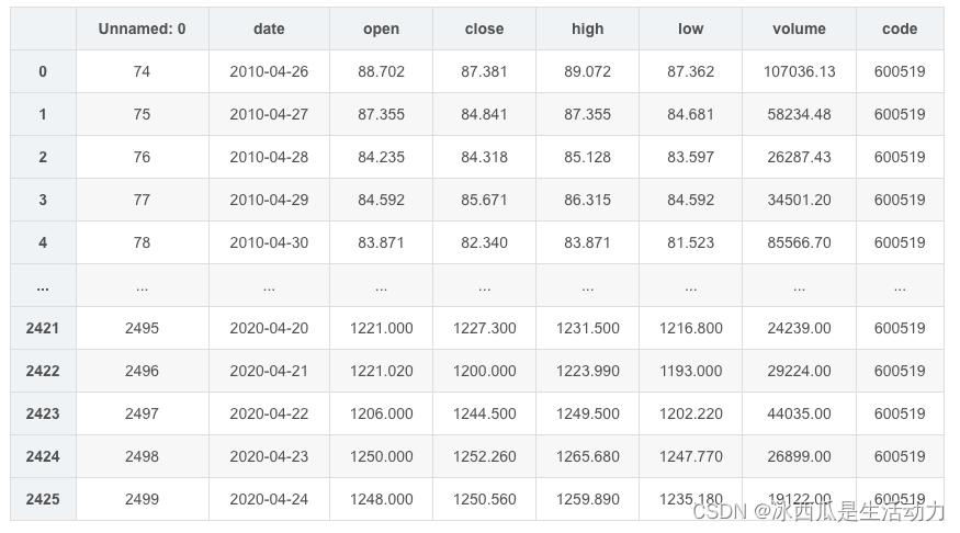
数据第二列是日期,第三列是开盘价格,数据集内含有2426条数据,通过学习其中一部分的数据,预测模型未看到过的模型。
二、学习内容
本节的一个特殊性是,股价是有周期性,而且每天的开盘价格不是独立事件,它会受前几天的股价影响的。针对这种预测任务,其实适合使用RNN网络。
1. 数据处理
"""
前(2426-300=2126)天的开盘价作为训练集,表格从0开始计数,2:3 是提取[2:3)列,前闭后开,故提取出C列开盘价
后300天的开盘价作为测试集
"""
training_set = data.iloc[0:2426 - 300, 2:3].values
test_set = data.iloc[2426 - 300:, 2:3].values

"""
归一化
"""
sc           = MinMaxScaler(feature_range=(0, 1))
training_set = sc.fit_transform(training_set)
test_set     = sc.transform(test_set)

x_train = []
y_train = []

x_test = []
y_test = []

"""
使用前60天的开盘价作为输入特征x_train
    第61天的开盘价作为输入标签y_train

for循环共构建2426-300-60=2066组训练数据。
       共构建300-60=260组测试数据
"""
for i in range(60, len(training_set)):
    x_train.append(training_set[i - 60:i, 0])
    y_train.append(training_set[i, 0])

for i in range(60, len(test_set)):
    x_test.append(test_set[i - 60:i, 0])
    y_test.append(test_set[i, 0])

# 对训练集进行打乱
np.random.seed(7)
np.random.shuffle(x_train)
np.random.seed(7)
np.random.shuffle(y_train)
tf.random.set_seed(7)

"""
将训练数据调整为数组(array)

调整后的形状:
x_train:(2066, 60, 1)
y_train:(2066,)
x_test :(240, 60, 1)
y_test :(240,)
"""
x_train, y_train = np.array(x_train), np.array(y_train) # x_train形状为:(2066, 60, 1)
x_test,  y_test  = np.array(x_test),  np.array(y_test)

"""
输入要求:[送入样本数, 循环核时间展开步数, 每个时间步输入特征个数]
"""
x_train = np.reshape(x_train, (x_train.shape[0], 60, 1))
x_test  = np.reshape(x_test,  (x_test.shape[0], 60, 1))
2. 建立神经网络
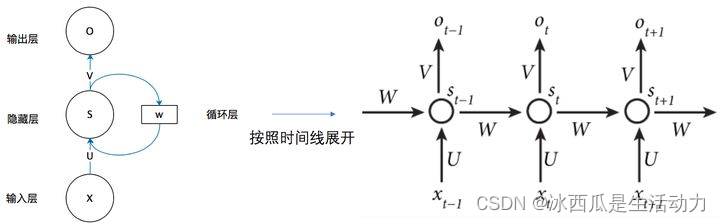
RNN网络最特别的一点就是前一次的状态会印象下一次的状态。
如下图所示,xt时刻的输入,经过线形得到st,再根据st做非线性的变换成为输出ot。
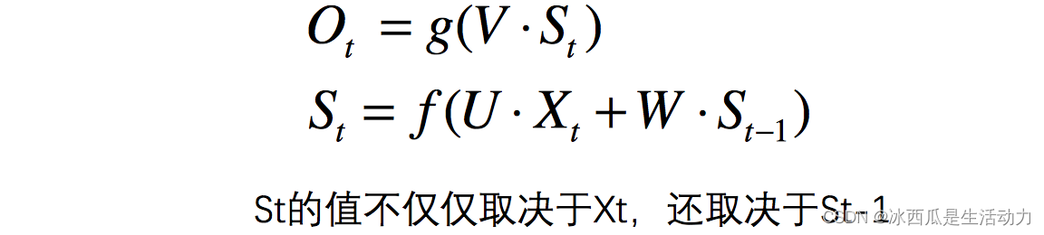
上面的这个介绍可能比较抽象,总结来说计算公式如下所示。
我看老师实际运用这个网络的时候就直接调用了接口。
model = tf.keras.Sequential([
    SimpleRNN(100, return_sequences=True), #布尔值。是返回输出序列中的最后一个输出,还是全部序列。
    Dropout(0.1),                         #防止过拟合
    SimpleRNN(100),
    Dropout(0.1),
    Dense(1)
])
但是其实这样学习不能真正感受到这个网络的结构,所以我专门找了一个手写rnn的例子,这个代码结合上面计算公式(主要看)
https://zhuanlan.zhihu.com/p/363932165
扫描二维码关注公众号,回复: 14486094 查看本文章
在RNN的class里
state = np.dot(self.Ux, inputX) + np.dot(self.Ws,self.stateList[times-1]) + self.Wb
这句就是上面的计算公式。
2.训练神经网络
训练过程,其实和之前做过的例子都没啥差别。
# 该应用只观测loss数值,不观测准确率,所以删去metrics选项,一会在每个epoch迭代显示时只显示loss值
model.compile(optimizer=tf.keras.optimizers.Adam(0.001),
              loss='mean_squared_error')  # 损失函数用均方误差
history = model.fit(x_train, y_train,
                    batch_size=64,
                    epochs=20,
                    validation_data=(x_test, y_test),
                    validation_freq=1)                  #测试的epoch间隔数

model.summary()
3.预测和模型评估
预测和评估也是和之前的练习相似。
history = model.fit(x_train, y_train,
batch_size=64,
epochs=20,
validation_data=(x_test, y_test),
validation_freq=1) #测试的epoch间隔数
model.summary()
predicted_stock_price = model.predict(x_test) # 测试集输入模型进行预测
predicted_stock_price = sc.inverse_transform(predicted_stock_price) # 对预测数据还原---从(0,1)反归一化到原始范围
real_stock_price = sc.inverse_transform(test_set[60:]) # 对真实数据还原---从(0,1)反归一化到原始范围
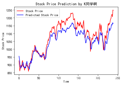
# 画出真实数据和预测数据的对比曲线
plt.plot(real_stock_price, color='red', label='Stock Price')
plt.plot(predicted_stock_price, color='blue', label='Predicted Stock Price')
plt.title('Stock Price Prediction by K同学啊')
plt.xlabel('Time')
plt.ylabel('Stock Price')
plt.legend()
plt.show()
比较特别的这里的模型评估,有一些特别的评估类型,以前我们遇到的情况,都是一个图片对应一个离散的结果,这样的情况是可以用准确率等方式评估,这次做的内容是连续值,那么描述连续值的相近成都就变成了MSE等等。
"""
MSE  :均方误差    ----->  预测值减真实值求平方后求均值
RMSE :均方根误差  ----->  对均方误差开方
MAE  :平均绝对误差----->  预测值减真实值求绝对值后求均值
R2   :决定系数,可以简单理解为反映模型拟合优度的重要的统计量

详细介绍可以参考文章:https://blog.csdn.net/qq_38251616/article/details/107997435
"""
MSE   = metrics.mean_squared_error(predicted_stock_price, real_stock_price)
RMSE  = metrics.mean_squared_error(predicted_stock_price, real_stock_price)**0.5
MAE   = metrics.mean_absolute_error(predicted_stock_price, real_stock_price)
R2    = metrics.r2_score(predicted_stock_price, real_stock_price)

print('均方误差: %.5f' % MSE)
print('均方根误差: %.5f' % RMSE)
print('平均绝对误差: %.5f' % MAE)
print('R2: %.5f' % R2)
总结
本章从预测股票出发,学习了RNN的一些基本概念。