手动实现一个扩散模型DDPM

扩散模型是目前大部分AIGC生图模型的基座，其本质是用神经网络学习从高斯噪声逐步恢复图像的过程，本文用python代码从零开始构建了一个简单的扩散模型。

理论部分

DDPM(Denoising Diffusion Probabilistic Models) 是一种在生成对抗网络等技术的基础上发展起来的新型概率模型去噪扩散模型，与其他生成模型（如归一化流、GANs或VAEs）相比并不是那么复杂，DDPM由两部分组成：

一个固定的前向传播的过程，它会逐渐将高斯噪声添加到图像中，直到最终得到纯噪声
一种可学习的反向去噪扩散过程，训练神经网络以从纯噪声开始逐渐对图像进行去噪

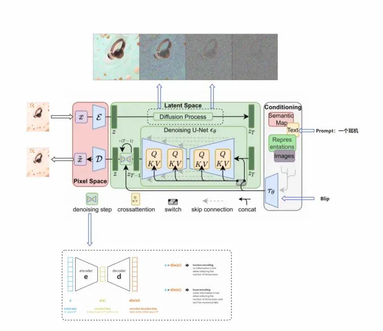
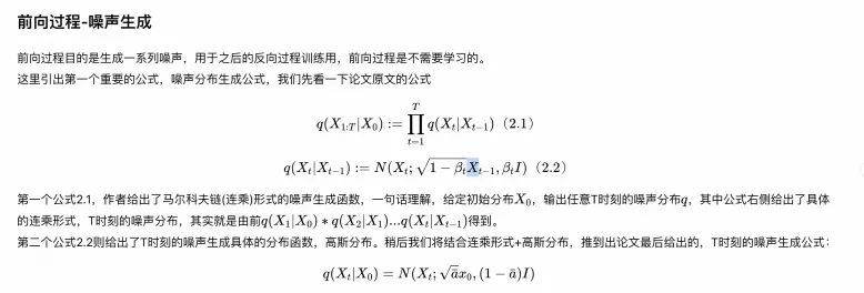
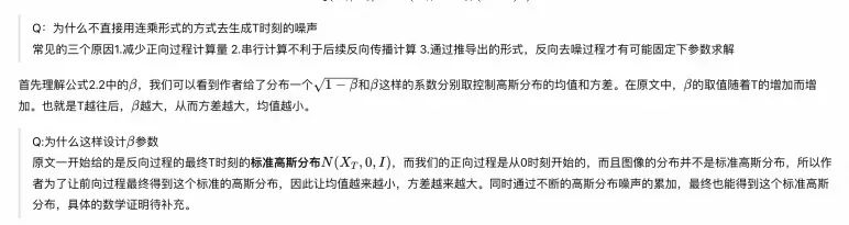
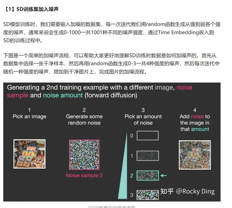
▐ 前向过程

前向扩散过程，其本质上是一个不断加噪声的过程。如下图所示，在猫的图片中多次增加高斯噪声直至图片变成随机噪音矩阵。可以看到，对于初始数据，我们设置K步的扩散步数，每一步增加一定的噪声，如果我们设置的K足够大，那么我们就能够将初始数据转化成随机噪音矩阵。

扫描二维码关注公众号，回复： 17384525 查看本文章

具体推理验证可参考： http://www.egbenz.com/#/my_article/12

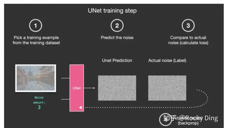
▐ 训练过程

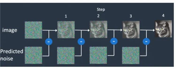
反向生成过程和前向扩散过程相反，是一个不断去噪的过程。神经网络从一个随机高斯噪声矩阵开始通过扩散模型的Inference过程不断预测并去除噪声。

实践部分

▐ 环境包

我们将首先安装并导入所需的库。

!pip install -q -U einops datasets matplotlib tqdm
import mathfrom inspect import isfunctionfrom functools import partial                                 
%matplotlib inlineimport matplotlib.pyplot as pltfrom tqdm.auto import tqdmfrom einops import rearrange, reducefrom einops.layers.torch import Rearrange
import torchfrom torch import nn, einsumimport torch.nn.functional as F

▐ 加噪声

下面是一些周期性的函数，这段代码定义了几种不同的函数，每个函数都用于计算深度学习中的beta调度（scheduling）。Beta调度主要用于控制噪声添加的程度，具体代码如下：

import torch
# cosine_beta_schedule函数用于创建一个余弦退火beta调度。# 这种调度方法基于余弦函数，并且可以调整随时间的衰减速率。def cosine_beta_schedule(timesteps, s=0.008):    steps = timesteps + 1  # 计算总的步数，需要比时间步多一个，以便计算alpha的累积乘积    x = torch.linspace(0, timesteps, steps)  # 创建从0到timesteps的均匀分布的张量    # 计算alpha的累积乘积，使用一个余弦变换，并平方来计算当前步的alpha值    alphas_cumprod = torch.cos(((x / timesteps) + s) / (1 + s) * torch.pi * 0.5) ** 2    alphas_cumprod = alphas_cumprod / alphas_cumprod[0]  # 归一化，确保初始值为1    betas = 1 - (alphas_cumprod[1:] / alphas_cumprod[:-1])  # 计算每个时间步的beta值    return torch.clip(betas, 0.0001, 0.9999)  # 对beta值进行裁剪，避免过大或过小
# linear_beta_schedule函数用于创建一个线性退火beta调度。# 这意味着beta值将从beta_start线性增加到beta_end。def linear_beta_schedule(timesteps):    beta_start = 0.0001  # 定义起始beta值    beta_end = 0.02  # 定义结束beta值    return torch.linspace(beta_start, beta_end, timesteps)  # 创建一个线性分布的beta值数组
# quadratic_beta_schedule函数用于创建一个二次退火beta调度。# 这意味着beta值将根据二次函数变化。def quadratic_beta_schedule(timesteps):    beta_start = 0.0001  # 定义起始beta值    beta_end = 0.02  # 定义结束beta值    # 创建一个线性分布的数组，然后将其平方以生成二次分布，最后再次平方以计算beta值    return torch.linspace(beta_start**0.5, beta_end**0.5, timesteps) ** 2
# sigmoid_beta_schedule函数用于创建一个sigmoid退火beta调度。# 这意味着beta值将根据sigmoid函数变化，这是一种常见的激活函数。def sigmoid_beta_schedule(timesteps):    beta_start = 0.0001  # 定义起始beta值    beta_end = 0.02  # 定义结束beta值    betas = torch.linspace(-6, 6, timesteps)  # 创建一个从-6到6的线性分布，用于sigmoid函数的输入    # 应用sigmoid函数，并根据beta_start和beta_end调整其范围和位置    return torch.sigmoid(betas) * (beta_end - beta_start) + beta_start

下面是噪声采样函数，其中extract 函数的作用是从预先计算的张量中提取适合当前时间步 t 的值。sqrt_alphas_cumprod 和 sqrt_one_minus_alphas_cumprod 应该是分别与时间关联的平方根累积乘积和其补数的平方根累积乘积，这两个张量中包含了不同时间步下噪声扩散的缩放系数。sqrt_alphas_cumprod_t * x_start 计算了经过时间步 t 缩放的原始数据，而 sqrt_one_minus_alphas_cumprod_t * noise 计算了同样经过时间步 t 缩放的噪声。两者相加得到的是在时间步 t 时刻的扩散数据。在扩散模型中，通过反向扩散过程（生成过程）来学习这种加噪声的逆过程，从而可以生成新的数据样本。

# import torch  # 假设在代码的其他部分已经导入了torch库
# 定义前向扩散函数# x_start: 初始数据，例如一批图像# t: 扩散的时间步，表示当前的扩散阶段# noise: 可选参数，如果提供，则使用该噪声数据；否则，将生成新的随机噪声def q_sample(x_start, t, noise=None):    if noise is None:        noise = torch.randn_like(x_start)  # 如果未提供噪声，则生成一个与x_start形状相同的随机噪声张量
    # 提取对应于时间步t的α的累积乘积的平方根    sqrt_alphas_cumprod_t = extract(sqrt_alphas_cumprod, t, x_start.shape)    # 提取对应于时间步t的1-α的累积乘积的平方根    sqrt_one_minus_alphas_cumprod_t = extract(        sqrt_one_minus_alphas_cumprod, t, x_start.shape    )
    # 返回前向扩散的结果，该结果是初始数据和噪声的线性组合    # 系数sqrt_alphas_cumprod_t和sqrt_one_minus_alphas_cumprod_t分别用于缩放初始数据和噪声    return sqrt_alphas_cumprod_t * x_start + sqrt_one_minus_alphas_cumprod_t * noise

测试如下：

# take time stepfor noise in [10,20,40,80 100]:  t = torch.tensor([40])  get_noisy_image(x_start, t)

▐ 核心残差网络

下面是残差网络的实现代码，Block 类是一个包含卷积、归一化、激活函数的标准神经网络层。ResnetBlock 类构建了一个残差块（residual block），这是深度残差网络（ResNet）的关键特性，它通过学习输入和输出的差异来提高网络性能。在 ResnetBlock 中，可选的 time_emb 参数和内部的 mlp 允许该Block处理与时间相关的特征。

import torch.nn as nnfrom einops import rearrange  # 假设已经导入了einops库中的rearrange函数from torch_utils import exists  # 假设已经定义了exists函数，用于检查对象是否存在
# 定义一个基础的Block类，该类将作为神经网络中的一个基本构建模块class Block(nn.Module):    def __init__(self, dim, dim_out, groups=8):        super().__init__()        # 一个2D卷积层，卷积核大小为3x3，边缘填充为1，从输入维度dim到输出维度dim_out        self.proj = nn.Conv2d(dim, dim_out, 3, padding=1)        # GroupNorm层用于归一化，分组数为groups        self.norm = nn.GroupNorm(groups, dim_out)        # 使用SiLU（也称为Swish）作为激活函数        self.act = nn.SiLU()            def forward(self, x, scale_shift=None):        x = self.proj(x)  # 应用卷积操作        x = self.norm(x)  # 应用归一化操作        # 如果scale_shift参数存在，则对归一化后的数据进行缩放和位移操作        if exists(scale_shift):            scale, shift = scale_shift            x = x * (scale + 1) + shift        x = self.act(x)  # 应用激活函数        return x  # 返回处理后的数据
# 定义一个ResnetBlock类，用于构建残差网络中的基本块class ResnetBlock(nn.Module):    """https://arxiv.org/abs/1512.03385"""        def __init__(self, dim, dim_out, *, time_emb_dim=None, groups=8):        super().__init__()        # 如果time_emb_dim存在，定义一个小型的多层感知器（MLP）网络        self.mlp = (            nn.Sequential(nn.SiLU(), nn.Linear(time_emb_dim, dim_out))            if exists(time_emb_dim)            else None        )        # 定义两个顺序的基础Block模块        self.block1 = Block(dim, dim_out, groups=groups)        self.block2 = Block(dim_out, dim_out, groups=groups)        # 如果输入维度dim和输出维度dim_out不同，则使用1x1卷积进行维度调整        # 否则使用Identity层（相当于不做任何处理）        self.res_conv = nn.Conv2d(dim, dim_out, 1) if dim != dim_out else nn.Identity()            def forward(self, x, time_emb=None):        h = self.block1(x)  # 通过第一个Block模块        # 如果存在时间嵌入向量time_emb且存在mlp模块，则将其应用到h上        if exists(self.mlp) and exists(time_emb):            time_emb = self.mlp(time_emb)  # 通过MLP网络            # 重整time_emb的形状以匹配h的形状，并将结果加到h上            h = rearrange(time_emb, "b c -> b c 1 1") + h        h = self.block2(h)  # 通过第二个Block模块        return h + self.res_conv(x)  # 将Block模块的输出与调整维度后的原始输入x相加并返回

▐ 注意力机制

DDPM的作者把大名鼎鼎的注意力机制加在卷积层之间。注意力机制是Transformer架构的基础模块(参考:Vaswani et al., 2017)，Transformer在AI各个领域，NLP,CV等等都取得了巨大的成功，这里Phil Wang实现了两个变种版本，一个是普通的多头注意力(用在了transformer中)，另一种是线性注意力机制(参考:Shen et al.,2018)，和普通的注意力在时间和存储的二次的增长相比，这个版本是线性增长的。

SelfAttention可以将输入图像的不同部分（像素或图像Patch）进行交互，从而实现特征的整合和全局上下文的引入，能够让模型建立捕捉图像全局关系的能力，有助于模型理解不同位置的像素之间的依赖关系，以更好地理解图像的语义。

在此基础上，SelfAttention还能减少平移不变性问题，SelfAttention模块可以在不考虑位置的情况下捕捉特征之间的关系，因此具有一定的平移不变性。

参考:Vaswani et al., 2017 地址：https://arxiv.org/abs/1706.03762

参考:Shen et al.,2018 地址：https://arxiv.org/abs/1812.01243

import torchfrom torch import nnfrom einops import rearrangeimport torch.nn.functional as F
# 定义一个标准的多头注意力（Multi-Head Attention）机制的类class Attention(nn.Module):    def __init__(self, dim, heads=4, dim_head=32):        super().__init__()        # 根据维度的倒数平方根来缩放查询（Query）向量        self.scale = dim_head ** -0.5        # 头的数量（多头中的"多"）        self.heads = heads        # 计算用于多头注意力的隐藏层维度        hidden_dim = dim_head * heads        # 定义一个卷积层将输入的特征映射到QKV（查询、键、值）空间        self.to_qkv = nn.Conv2d(dim, hidden_dim * 3, 1, bias=False)        # 定义一个卷积层将多头注意力的输出映射回原特征空间        self.to_out = nn.Conv2d(hidden_dim, dim, 1)
    def forward(self, x):        # 获取输入的批量大小、通道数、高度和宽度        b, c, h, w = x.shape        # 使用to_qkv卷积层得到QKV，并将其分离为三个组件        qkv = self.to_qkv(x).chunk(3, dim=1)        # 将QKV重排并缩放查询向量        q, k, v = map(            lambda t: rearrange(t, "b (h c) x y -> b h c (x y)", h=self.heads), qkv        )        q = q * self.scale        # 使用爱因斯坦求和约定计算查询和键之间的相似度得分        sim = einsum("b h d i, b h d j -> b h i j", q, k)        # 从相似度得分中减去最大值以提高数值稳定性        sim = sim - sim.amax(dim=-1, keepdim=True).detach()        # 应用Softmax函数获取注意力权重        attn = sim.softmax(dim=-1)        # 使用注意力权重对值进行加权        out = einsum("b h i j, b h d j -> b h i d", attn, v)        # 将输出重新排列回原始的空间形状        out = rearrange(out, "b h (x y) d -> b (h d) x y", x=h, y=w)        # 返回通过输出卷积层的结果        return self.to_out(out)
# 定义一个线性注意力（Linear Attention）机制的类class LinearAttention(nn.Module):    def __init__(self, dim, heads=4, dim_head=32):        super().__init__()        # 根据维度的倒数平方根来缩放查询（Query）向量        self.scale = dim_head ** -0.5        # 头的数量        self.heads = heads        # 计算用于多头注意力的隐藏层维度        hidden_dim = dim_head * heads        # 定义一个卷积层将输入的特征映射到QKV空间        self.to_qkv = nn.Conv2d(dim, hidden_dim * 3, 1, bias=False)        # 定义一个顺序容器包含卷积层和组归一化层将输出映射回原特征空间        self.to_out = nn.Sequential(nn.Conv2d(hidden_dim, dim, 1),                                    nn.GroupNorm(1, dim))
    def forward(self, x):        # 获取输入的批量大小、通道数、高度和宽度        b, c, h, w = x.shape        # 使用to_qkv卷积层得到QKV，并将其分离为三个组件        qkv = self.to_qkv(x).chunk(3, dim=1)        # 将QKV重排，应用Softmax函数并缩放查询向量        q, k, v = map(            lambda t: rearrange(t, "b (h c) x y -> b h c (x y)", h=self.heads), qkv        )        q = q.softmax(dim=-2)        k = k.softmax(dim=-1)        q = q * self.scale        # 计算上下文矩阵，是键和值的加权组合        context = torch.einsum("b h d n, b h e n -> b h d e", k, v)        # 使用上下文矩阵和查询计算最终的注意力输出        out = torch.einsum("b h d e, b h d n -> b h e n", context, q)        # 将输出重新排列回原始的空间形状        out = rearrange(out, "b h c (x y) -> b (h c) x y", h=self.heads, x=h, y=w)        # 返回经过输出顺序容器处理的结果        return self.to_out(out)

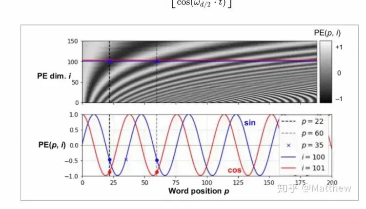
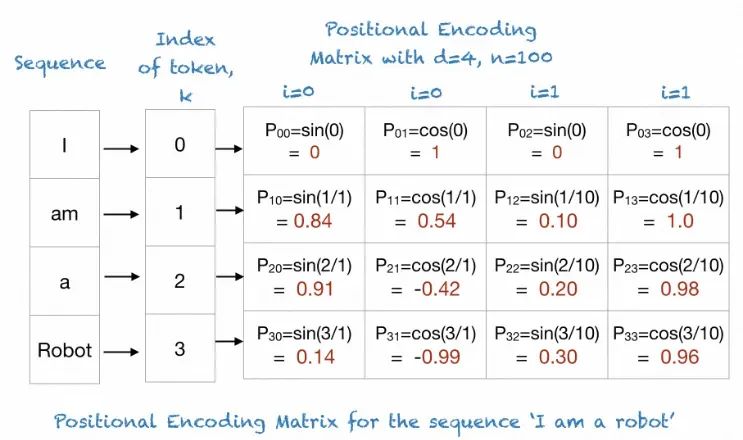
▐ 位置嵌入

如何让网络知道目前处于K的哪一步？可以增加一个Time Embedding（类似于Positional embeddings）进行处理，通过将timestep编码进网络中，从而只需要训练一个共享的U-Net模型，就可以让网络知道现在处于哪一步了。

Time Embedding正是输入到ResNetBlock模块中，为U-Net引入了时间信息（时间步长T，T的大小代表了噪声扰动的强度），模拟一个随时间变化不断增加不同强度噪声扰动的过程，让SD模型能够更好地理解时间相关性。

同时，在SD模型调用U-Net重复迭代去噪的过程中，我们希望在迭代的早期，能够先生成整幅图片的轮廓与边缘特征，随着迭代的深入，再补充生成图片的高频和细节特征信息。由于在每个ResNetBlock模块中都有Time Embedding，就能告诉U-Net现在是整个迭代过程的哪一步，并及时控制U-Net够根据不同的输入特征和迭代阶段而预测不同的噪声残差。

从AI绘画应用视角解释一下Time Embedding的作用。Time Embedding能够让SD模型在生成图片时考虑时间的影响，使得生成的图片更具有故事性、情感和沉浸感等艺术效果。并且Time Embedding可以帮助SD模型在不同的时间点将生成的图片添加完善不同情感和主题的内容，从而增加了AI绘画的多样性和表现力。

class SinusoidalPositionEmbeddings(nn.Module):    def __init__(self, dim):        super().__init__()        self.dim = dim
    def forward(self, time):        device = time.device        half_dim = self.dim // 2        embeddings = math.log(10000) / (half_dim - 1)        embeddings = torch.exp(torch.arange(half_dim, device=device) * -embeddings)        embeddings = time[:, None] * embeddings[None, :]        embeddings = torch.cat((embeddings.sin(), embeddings.cos()), dim=-1)        return embeddings

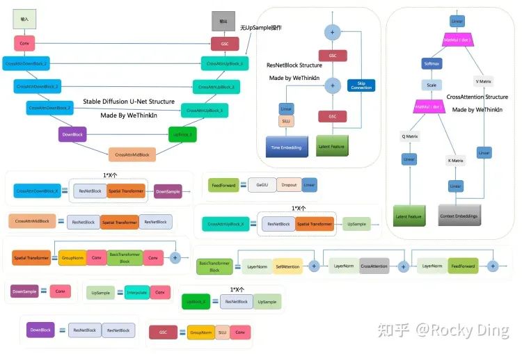
▐ U-net

基于上述定义的DM神经网络基础的层和模块，现在是时候把他组装拼接起来了：

神经网络接受一批如下shape的噪声图像输入(batch_size, num_channels, height, width) 同时接受这批噪声水平,shape=(batch_size, 1)。返回一个张量，shape = (batch_size, num_channels, height, width)

按照如下步骤构建这个网络：

首先，对噪声图像进行卷积处理，对噪声水平进行进行位置编码（embedding）
然后，进入一个序列的下采样阶段，每个下采样阶段由两个ResNet/ConvNeXT模块+分组归一化+注意力模块+残差链接+下采样完成。
在网络的中间层，再一次用ResNet/ConvNeXT模块，中间穿插着注意力模块(Attention)。
下一个阶段，则是序列构成的上采样阶段，每个上采样阶段由两个ResNet/ConvNeXT模块+分组归一化+注意力模块+残差链接+上采样完成。
最后，一个ResNet/ConvNeXT模块后面跟着一个卷积层。

class Unet(nn.Module):    # 初始化函数，定义U-Net网络的结构和参数    def __init__(            self,            dim,  # 基本隐藏层维度            init_dim=None,  # 初始层维度，如果未提供则会根据dim计算得出            out_dim=None,  # 输出维度，如果未提供则默认为输入图像的通道数            dim_mults=(1, 2, 4, 8),  # 控制每个阶段隐藏层维度倍增的倍数            channels=3,  # 输入图像的通道数，默认为3            with_time_emb=True,  # 是否使用时间嵌入，这对于某些生成模型可能是必要的            resnet_block_groups=8,  # ResNet块中的组数            use_convnext=True,  # 是否使用ConvNeXt块而不是ResNet块            convnext_mult=2,  # ConvNeXt块的维度倍增因子    ):        super().__init__()  # 调用父类构造函数        # 确定各层维度        self.channels = channels        init_dim = default(init_dim, dim // 3 * 2)  # 设置或计算初始层维度        self.init_conv = nn.Conv2d(channels, init_dim, 7, padding=3)  # 初始卷积层，使用7x7卷积核和padding        dims = [init_dim, *map(lambda m: dim * m, dim_mults)]  # 计算每个阶段的维度        in_out = list(zip(dims[:-1], dims[1:]))  # 创建输入输出维度对        # 根据use_convnext选择块类        if use_convnext:            block_klass = partial(ConvNextBlock, mult=convnext_mult)        else:            block_klass = partial(ResnetBlock, groups=resnet_block_groups)        # 时间嵌入层        if with_time_emb:            time_dim = dim * 4  # 时间嵌入的维度            self.time_mlp = nn.Sequential(  # 时间嵌入的多层感知机                SinusoidalPositionEmbeddings(dim),  # 正弦位置嵌入                nn.Linear(dim, time_dim),  # 线性变换                nn.GELU(),  # GELU激活函数                nn.Linear(time_dim, time_dim),  # 再一次线性变换            )        else:            time_dim = None            self.time_mlp = None        # 下采样层        self.downs = nn.ModuleList([])        self.ups = nn.ModuleList([])        num_resolutions = len(in_out)  # 解析的层数        # 构建下采样模块        for ind, (dim_in, dim_out) in enumerate(in_out):            is_last = ind >= (num_resolutions - 1)  # 是否为最后一层            self.downs.append(  # 添加下采样块                nn.ModuleList(                    [                        block_klass(dim_in, dim_out, time_emb_dim=time_dim),  # 卷积块                        block_klass(dim_out, dim_out, time_emb_dim=time_dim),  # 卷积块                        Residual(PreNorm(dim_out, LinearAttention(dim_out))),  # 残差连接和注意力模块                        Downsample(dim_out) if not is_last else nn.Identity(),  # 下采样或恒等映射                    ]                )            )        # 中间层（瓶颈层）        mid_dim = dims[-1]        # 中间层（瓶颈层）        # 第一个中间卷积块        self.mid_block1 = block_klass(mid_dim, mid_dim, time_emb_dim=time_dim)        # 中间层的注意力模块        self.mid_attn = Residual(PreNorm(mid_dim, Attention(mid_dim)))        # 第二个中间卷积块        self.mid_block2 = block_klass(mid_dim, mid_dim, time_emb_dim=time_dim)
        # 构建上采样模块        for ind, (dim_in, dim_out) in enumerate(reversed(in_out[1:])):            is_last = ind >= (num_resolutions - 1)  # 是否是最后一次上采样，减2是因为我们需要留出一个输出层            self.ups.append(                nn.ModuleList(                    [                        # 卷积块，这里输入维度翻倍是因为上采样过程中会与编码器阶段的相应层进行拼接                        block_klass(dim_out * 2, dim_in, time_emb_dim=time_dim),                        # 卷积块                        block_klass(dim_in, dim_in, time_emb_dim=time_dim),                        # 残差和注意力模块                        Residual(PreNorm(dim_in, LinearAttention(dim_in))),                        # 上采样或恒等映射                        Upsample(dim_in) if not is_last else nn.Identity(),                    ]                )            )
        # 设置或计算输出维度，如果未提供则默认为输入图像的通道数        out_dim = default(out_dim, channels)        # 最后的卷积层，将输出维度变换到期望的输出维度        self.final_conv = nn.Sequential(            block_klass(dim, dim),  # 卷积块            nn.Conv2d(dim, out_dim, 1)  # 1x1卷积，用于输出维度变换        )
    # 前向传播函数    def forward(self, x, time):        # 初始卷积层        x = self.init_conv(x)        # 如果存在时间嵌入层，则将时间编码        t = self.time_mlp(time) if exists(self.time_mlp) else None        # 用于存储各个阶段的特征图        h = []
        # 下采样过程        for block1, block2, attn, downsample in self.downs:            x = block1(x, t)  # 应用卷积块            x = block2(x, t)  # 应用卷积块            x = attn(x)  # 应用注意力模块            h.append(x)  # 存储特征图以便后续的拼接            x = downsample(x)  # 应用下采样或恒等映射
        # 中间层或瓶颈层        x = self.mid_block1(x, t)  # 第一个中间卷积块        x = self.mid_attn(x)  # 中间层的注意力模块        x = self.mid_block2(x, t)  # 第二个中间卷积块
        # 上采样过程        for block1, block2, attn, upsample in self.ups:            # 拼接特征图和对应的编码器阶段的特征图            x = torch.cat((x, h.pop()), dim=1)            x = block1(x, t)  # 应用卷积块            x = block2(x, t)  # 应用卷积块            x = attn(x)  # 应用注意力模块            x = upsample(x)  # 应用上采样或恒等映射
        # 最后的输出层，输出最终的特征图或图像        return self.final_conv(x)

▐ 损失函数

下面这段代码是为扩散模型中的去噪模型定义的损失函数。它计算由去噪模型预测的噪声和实际加入的噪声之间的差异。该函数支持不同类型的损失，包括L1损失、均方误差损失（L2损失）和Huber损失。选择适当的损失函数可以帮助模型更好地学习如何预测和去除生成数据中的噪声。

import torchimport torch.nn.functional as F
# 定义损失函数，它评估去噪模型的性能def p_losses(denoise_model, x_start, t, noise=None, loss_type="l1"):    if noise is None:        noise = torch.randn_like(x_start)  # 如果未提供噪声，则生成一个与x_start形状相同的随机噪声张量
    # 使用q_sample函数生成带有噪声的数据x_noisy，这模拟了扩散模型的前向过程    x_noisy = q_sample(x_start=x_start, t=t, noise=noise)    # 使用去噪模型对噪声数据x_noisy进行预测，试图恢复加入的噪声    predicted_noise = denoise_model(x_noisy, t)
    # 根据指定的损失类型计算损失    if loss_type == 'l1':  # 如果损失类型为L1损失        loss = F.l1_loss(noise, predicted_noise)  # 使用L1损失函数计算真实噪声和预测噪声之间的差异    elif loss_type == 'l2':  # 如果损失类型为L2损失（均方误差损失）        loss = F.mse_loss(noise, predicted_noise)  # 使用均方误差损失函数计算真实噪声和预测噪声之间的差异    elif loss_type == "huber":  # 如果损失类型为Huber损失        loss = F.smooth_l1_loss(noise, predicted_noise)  # 使用Huber损失函数，这是L1和L2损失的结合，对异常值不那么敏感    else:        raise NotImplementedError()  # 如果指定了未实现的损失类型，则抛出异常
    return loss  # 返回计算得到的损失值

▐ 开始训练

if __name__=="__main__":    for epoch in range(epochs):        for step, batch in tqdm(enumerate(dataloader), desc='Training'):          optimizer.zero_grad()          batch = batch[0]
          batch_size = batch.shape[0]          batch = batch.to(device)          # 国内版启用这段，注释上面两行          # batch_size = batch[0].shape[0]          # batch = batch[0].to(device)
          # Algorithm 1 line 3: sample t uniformally for every example in the batch          t = torch.randint(0, timesteps, (batch_size,), device=device).long()
          loss = p_losses(model, batch, t, loss_type="huber")
          if step % 50 == 0:            print("Loss:", loss.item())
          loss.backward()          optimizer.step()
          # save generated images          if step != 0 and step % save_and_sample_every == 0:            milestone = step // save_and_sample_every            batches = num_to_groups(4, batch_size)            all_images_list = list(map(lambda n: sample(model, batch_size=n, channels=channels), batches))            all_images = torch.cat(all_images_list, dim=0)            all_images = (all_images + 1) * 0.5            # save_image(all_images, str(results_folder / f'sample-{milestone}.png'), nrow = 6)            currentDateAndTime = datetime.now()            torch.save(model,f"train.pt")

▐ 推理结果

参考文献

深入学习：Diffusion Model 原理解析（地址：http://www.egbenz.com/#/my_article/12）
【一个本子】Diffusion Model 原理详解（地址：https://zhuanlan.zhihu.com/p/582072317）
深入浅出扩散模型(Diffusion Model)系列：基石DDPM（模型架构篇），最详细的DDPM架构图解（地址：https://zhuanlan.zhihu.com/p/637815071）
一文读懂Transformer模型的位置编码（地址：https://zhuanlan.zhihu.com/p/637815071
https://zhuanlan.zhihu.com/p/632809634

团队介绍

我们是淘天集团业务技术线的手猫营销&导购团队，专注于在手机天猫平台上探索创新商业化，我们依托淘天集团强大的互联网背景，致力于为手机天猫平台提供效率高、创新性强的技术支持。
我们的队员们来自各种营销和导购领域，拥有丰富的经验。通过不断地技术探索和商业创新，我们改善了用户的体验，并提升了平台的运营效率。
我们的团队持续不懈地探索和提升技术能力，坚持“技术领先、用户至上”，为手机天猫的导购场景和商业发展做出了显著贡献。

¤ 拓展阅读 ¤

3DXR技术 | 终端技术 | 音视频技术

服务端技术 | 技术质量 | 数据算法

本文分享自微信公众号 - 大淘宝技术（AlibabaMTT）。
如有侵权，请联系 [email protected] 删除。
本文参与“OSC源创计划”，欢迎正在阅读的你也加入，一起分享。