经典CNN卷积神经网络架构全解析:LeNet、AlexNet、GoogleNet、ResNet、DenseNet
卷积神经网络 (CNN)是深度学习中的一种神经网络架构,用于从结构化数组中识别模式。然而,多年来,CNN 架构已经发展起来。基本 CNN 架构的许多变体已经开发出来,从而为不断发展的深度学习领域带来了惊人的进步。
下面,让我们讨论一下 CNN 架构是如何随着时间的推移而发展和成长的。
1.LeNet-5
-
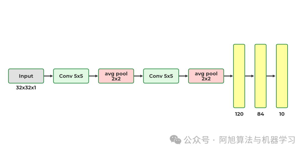
第一个LeNet-5架构是最广为人知的CNN架构。它于1998年推出,广泛用于手写方法数字识别。
-
LeNet-5 有 2 个卷积层和 3 个完整层。
-
这个LeNet-5架构有60,000个参数。结构如下:
-
LeNet-5 能够处理需要更大、更多 CNN 卷积层的更高分辨率图像。
-
leNet-5 技术是通过所有计算资源的可用性来衡量的
LeNet-5网络构建
LeNet-5 代码示例
import torch
from torchsummary import summary
import torch.nn as nn
import torch.nn.functional as F class LeNet5(nn.Module):
 def __init__(self):
  # Call the parent class's init method
  super(LeNet5, self).__init__()     # First Convolutional Layer
  self.conv1 = nn.Conv2d(in_channels=1, out_channels=6, kernel_size=5, stride=1)     # Max Pooling Layer
  self.pool = nn.MaxPool2d(kernel_size=2, stride=2)     # Second Convolutional Layer
  self.conv2 = nn.Conv2d(in_channels=6, out_channels=16, kernel_size=5, stride=1)     # First Fully Connected Layer
  self.fc1 = nn.Linear(in_features=16 * 5 * 5, out_features=120)     # Second Fully Connected Layer
  self.fc2 = nn.Linear(in_features=120, out_features=84)     # Output Layer
  self.fc3 = nn.Linear(in_features=84, out_features=10)  def forward(self, x):
  # Pass the input through the first convolutional layer and activation function
  x = self.pool(F.relu(self.conv1(x)))     # Pass the output of the first layer through
  # the second convolutional layer and activation function
  x = self.pool(F.relu(self.conv2(x)))     # Reshape the output to be passed through the fully connected layers
  x = x.view(-1, 16 * 5 * 5)     # Pass the output through the first fully connected layer and activation function
  x = F.relu(self.fc1(x))     # Pass the output of the first fully connected layer through
  # the second fully connected layer and activation function
  x = F.relu(self.fc2(x))     # Pass the output of the second fully connected layer through the output layer
  x = self.fc3(x)     # Return the final output
  return x  lenet5 = LeNet5()
print(lenet5)
输出:
LeNet5(
  (conv1): Conv2d(1, 6, kernel_size=(5, 5), stride=(1, 1))
  (pool): MaxPool2d(kernel_size=2, stride=2, padding=0, dilation=1, ceil_mode=False)
  (conv2): Conv2d(6, 16, kernel_size=(5, 5), stride=(1, 1))
  (fc1): Linear(in_features=400, out_features=120, bias=True)
  (fc2): Linear(in_features=120, out_features=84, bias=True)
  (fc3): Linear(in_features=84, out_features=10, bias=True)
)
lenet5模型概要
打印 lenet5 的summary 来检查参数
# add the cuda to the mode
device = torch.device("cuda" if torch.cuda.is_available() else "cpu")
lenet5.to(device) #Print the summary of the model
summary(lenet5, (1, 32, 32))
输出:

----------------------------------------------------------------
        Layer (type)               Output Shape         Param #
================================================================
            Conv2d-1            [-1, 6, 28, 28]             156
         MaxPool2d-2            [-1, 6, 14, 14]               0
            Conv2d-3           [-1, 16, 10, 10]           2,416
         MaxPool2d-4             [-1, 16, 5, 5]               0
            Linear-5                  [-1, 120]          48,120
            Linear-6                   [-1, 84]          10,164
            Linear-7                   [-1, 10]             850
================================================================
Total params: 61,706
Trainable params: 61,706
Non-trainable params: 0
----------------------------------------------------------------
Input size (MB): 0.00
Forward/backward pass size (MB): 0.06
Params size (MB): 0.24
Estimated Total Size (MB): 0.30
----------------------------------------------------------------
2. AlexNNet
-
AlexNet CNN 架构在 2012 年 ImageNet ILSVRC 深度学习算法挑战赛中以较大的方差获胜,达到了 17%,而排名第二的 top-5 错误率达到了 26%!
-
它是由 Alex Krizhevsky(创始人姓名)、Ilya Sutskever 和 Geoffrey Hinton 引入的,与 LeNet-5 非常相似,只是更大更深,并且它首先被引入将卷积层直接堆叠在彼此模型之上,而不是在 CN 网络卷积层上堆叠一个池化层。
-
AlexNNet 有 6000 万个参数,因为 AlexNet 总共有 8 层,5 个卷积层和 3 个全连接层。
-
AlexNNet 首次将(ReLU)整流线性单元作为激活函数
-
这是第一个使用GPU来提高性能的CNN架构。
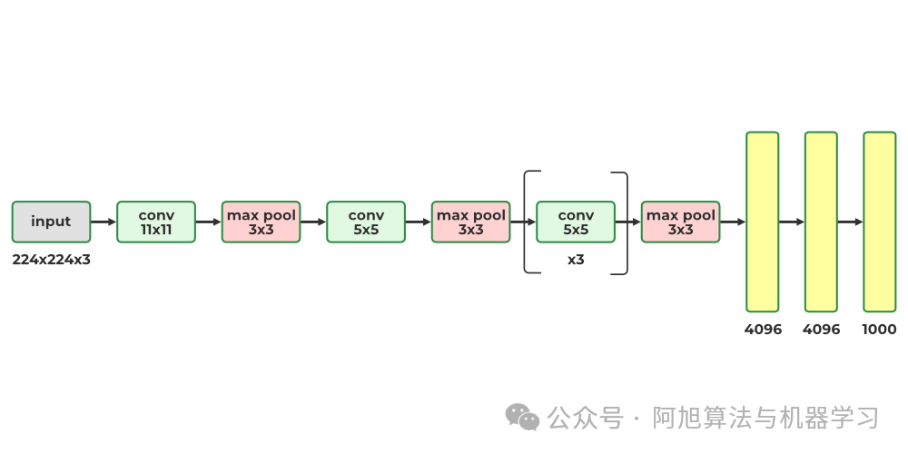
ALexNNet - Geeksforgeeks
AlexNNet模型构建
AlexNNet 的构建模型代码:
import torch
from torchsummary import summary
import torch.nn as nn
import torch.nn.functional as F class AlexNet(nn.Module):
 def __init__(self, num_classes=1000):
  # Call the parent class's init method to initialize the base class
  super(AlexNet, self).__init__()     # First Convolutional Layer with 11x11 filters, stride of 4, and 2 padding
  self.conv1 = nn.Conv2d(in_channels=3, out_channels=96, kernel_size=11, stride=4, padding=2)     # Max Pooling Layer with a kernel size of 3 and stride of 2
  self.pool = nn.MaxPool2d(kernel_size=3, stride=2)     # Second Convolutional Layer with 5x5 filters and 2 padding
  self.conv2 = nn.Conv2d(in_channels=96, out_channels=256, kernel_size=5, padding=2)     # Third Convolutional Layer with 3x3 filters and 1 padding
  self.conv3 = nn.Conv2d(in_channels=256, out_channels=384, kernel_size=3, padding=1)     # Fourth Convolutional Layer with 3x3 filters and 1 padding
  self.conv4 = nn.Conv2d(in_channels=384, out_channels=384, kernel_size=3, padding=1)     # Fifth Convolutional Layer with 3x3 filters and 1 padding
  self.conv5 = nn.Conv2d(in_channels=384, out_channels=256, kernel_size=3, padding=1)     # First Fully Connected Layer with 4096 output features
  self.fc1 = nn.Linear(in_features=256 * 6 * 6, out_features=4096)     # Second Fully Connected Layer with 4096 output features
  self.fc2 = nn.Linear(in_features=4096, out_features=4096)     # Output Layer with `num_classes` output features
  self.fc3 = nn.Linear(in_features=4096, out_features=num_classes)  def forward(self, x):
  # Pass the input through the first convolutional layer and ReLU activation function
  x = self.pool(F.relu(self.conv1(x)))     # Pass the output of the first layer through
  # the second convolutional layer and ReLU activation function
  x = self.pool(F.relu(self.conv2(x)))     # Pass the output of the second layer through
  # the third convolutional layer and ReLU activation function
  x = F.relu(self.conv3(x))     # Pass the output of the third layer through
  # the fourth convolutional layer and ReLU activation function
  x = F.relu(self.conv4(x))     # Pass the output of the fourth layer through
  # the fifth convolutional layer and ReLU activation function
  x = self.pool(F.relu(self.conv5(x)))     # Reshape the output to be passed through the fully connected layers
  x = x.view(-1, 256 * 6 * 6)     # Pass the output through the first fully connected layer and activation function
  x = F.relu(self.fc1(x))
  x = F.dropout(x, 0.5)      # Pass the output of the first fully connected layer through
  # the second fully connected layer and activation function
  x = F.relu(self.fc2(x))     # Pass the output of the second fully connected layer through the output layer
  x = self.fc3(x)     # Return the final output
  return x                     alexnet = AlexNet()
print(alexnet)
输出:
AlexNet(
  (conv1): Conv2d(3, 96, kernel_size=(11, 11), stride=(4, 4), padding=(2, 2))
  (pool): MaxPool2d(kernel_size=3, stride=2, padding=0, dilation=1, ceil_mode=False)
  (conv2): Conv2d(96, 256, kernel_size=(5, 5), stride=(1, 1), padding=(2, 2))
  (conv3): Conv2d(256, 384, kernel_size=(3, 3), stride=(1, 1), padding=(1, 1))
  (conv4): Conv2d(384, 384, kernel_size=(3, 3), stride=(1, 1), padding=(1, 1))
  (conv5): Conv2d(384, 256, kernel_size=(3, 3), stride=(1, 1), padding=(1, 1))
  (fc1): Linear(in_features=9216, out_features=4096, bias=True)
  (fc2): Linear(in_features=4096, out_features=4096, bias=True)
  (fc3): Linear(in_features=4096, out_features=1000, bias=True)
)
模型概要
打印 alexnet 的summary以查看模型参数:
# add the cuda to the mode
device = torch.device("cuda" if torch.cuda.is_available() else "cpu")
alexnet.to(device) #Print the summary of the model
summary(alexnet, (3, 224, 224))
输出:
----------------------------------------------------------------
        Layer (type)               Output Shape         Param #
================================================================
            Conv2d-1           [-1, 96, 55, 55]          34,944
         MaxPool2d-2           [-1, 96, 27, 27]               0
            Conv2d-3          [-1, 256, 27, 27]         614,656
         MaxPool2d-4          [-1, 256, 13, 13]               0
            Conv2d-5          [-1, 384, 13, 13]         885,120
            Conv2d-6          [-1, 384, 13, 13]       1,327,488
            Conv2d-7          [-1, 256, 13, 13]         884,992
         MaxPool2d-8            [-1, 256, 6, 6]               0
            Linear-9                 [-1, 4096]      37,752,832
           Linear-10                 [-1, 4096]      16,781,312
           Linear-11                 [-1, 1000]       4,097,000
================================================================
Total params: 62,378,344
Trainable params: 62,378,344
Non-trainable params: 0
----------------------------------------------------------------
Input size (MB): 0.57
Forward/backward pass size (MB): 5.96
Params size (MB): 237.95
Estimated Total Size (MB): 244.49
----------------------------------------------------------------
3. GoogleNet(Inception vl)
-
GoogleNet架构由 Google Research 的 Christian Szegedy 创建,并在 ILSVRC 2014 挑战赛中将前五名错误率降低到 7% 以下,取得了突破性成果。这一成功很大程度上归功于其比其他 CNN 更深的架构,这得益于其初始模块,与之前的架构相比,该模块能够更有效地使用参数 -
GoogleNet 的参数比 AlexNet 少,比例为 10:1(大约 600 万而不是 6000 万)
-
Inception 模块的架构如图所示。

GoogleNet(Inception 模块) - Geeksforgeeks
GoogleNet(Inception 模块)
-
符号“3 x 3 + 2(5)”表示该层使用 3 x 3 内核、步幅为 2 和 SAME 填充。输入信号随后被馈送到四个不同的层,每个层都具有 RelU 激活函数和步幅为 1。这些卷积层具有不同的内核大小(1 x 1、3 x 3 和 5 x 5),以捕获不同尺度的模式。此外,每个层都使用 SAME 填充,因此所有输出都具有与其输入相同的高度和宽度。这允许将来自所有四个顶部卷积层的特征图沿最终深度连接层中的深度维度连接起来。
-
整体 GoogleNet 架构有 22 个较大的深度 CNN 层。
4.ResNet(残差网络)
-
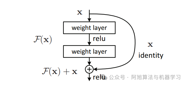
残差网络 (ResNet)是 ILSVRC 2015 挑战赛的获胜者,由 Kaiming He 开发,其 CNN 深度极深,由 152 层组成,前五名错误率高达 3.6%。训练如此深度网络的一个重要因素是使用跳跃连接(也称为快捷连接)。进入某一层的信号被添加到堆栈中更高层的输出中。让我们来探索一下为什么这样做是有益的。 -
训练神经网络时,目标是让它复制目标函数 h(x)。通过将输入 x 添加到网络的输出(跳过连接),网络可以建模 f(x) = h(x) – x,这种技术称为残差学习。
F(x) = H(x) - x得出H(x) := F(x) + x。
ResNet(残差网络) - Geeksforgeeks
跳跃(快捷方式)连接
-
初始化常规神经网络时,其权重接近于零,导致网络输出接近于零的值。通过添加跳跃连接,生成的网络将输出其输入的副本,从而有效地对恒等函数进行建模。如果目标函数与恒等函数相似,这将大有裨益,因为它将加速训练。此外,如果添加多个跳跃连接,即使多个层尚未开始学习,网络也可以开始取得进展。
-
目标函数非常接近identity函数(通常情况如此),这将大大加快训练速度。
-
深度残差网络可以看作是一系列残差单元,每个残差单元都是一个带有跳跃连接的小型神经网络
5. DenseNet
-
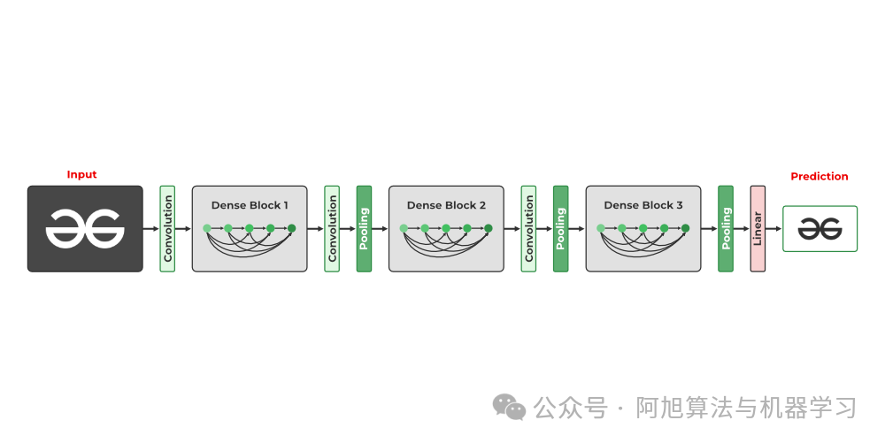
DenseNet模型引入了密集连接的卷积网络的概念,其中每一层的输出都连接到每个后续层的输入。这一设计原则是为了解决高级神经网络中梯度消失和梯度爆炸导致的准确率下降问题而提出的。 -
简单来说,由于输入层和输出层之间的距离太远,数据在到达目的地之前就丢失了。
-
DenseNet 模型引入了密集连接的卷积网络的概念,其中每一层的输出都连接到每个后续层的输入。这一设计原则是为了解决高级神经网络中梯度消失和梯度爆炸导致的准确率下降问题而提出的。
DenseNet - Geeksforgeeks
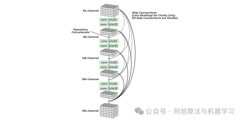
密集网络
-
密集块中的所有卷积均由 ReLU 激活并使用批量归一化。仅当数据的高度和宽度尺寸保持不变时,才可以进行通道级联,因此密集块中的卷积均为步长 1。池化层插入密集块之间以进一步降低维度。
-
直观地看,人们可能会认为,通过连接所有之前看到的输出,通道和参数的数量将呈指数级增长。然而,DenseNet 在可学习参数方面出奇地经济。这是因为每个连接的块(可能具有相对大量的通道)首先通过 1×1 卷积,将其减少到较少的通道数。此外,1×1 卷积在参数方面是经济的。然后,应用具有相同通道数的 3×3 卷积。
-
DenseNet 每个步骤产生的通道都连接到所有先前生成的输出的集合。每个步骤都利用一对 1×1 和 3×3 卷积,为数据添加 K 个通道。因此,通道数量随着密集块中的卷积步骤数量线性增加。整个网络的增长率保持不变,DenseNet 在 K 值介于 12 到 40 之间时表现出良好的性能。
-
密集块和池化层组合起来形成 Tu DenseNet 网络。DenseNet21 有 121 层,但结构可调整,可轻松扩展到 200 层以上