在使用 AMD GPU 的 PyTorch 中实现自动混合精度

Automatic mixed precision in PyTorch using AMD GPUs — ROCm Blogs

随着模型规模的增加，训练它们所需的时间和内存——以及因此而产生的成本——也在增加。因此，采取任何措施来减少训练时间和内存使用都是非常有益的。这就是自动混合精度（AMP）派上用场的地方。

在这篇博文中，我们将讨论 AMP 的基础知识、其工作原理以及它如何提高 AMD GPU 上的训练效率。

前提条件

要运行本博客中使用的代码，您需要以下内容：

• 硬件

  • AMD GPU - 请参阅兼容 GPU 列表

  操作系统

  • Linux - 请参阅支持的 Linux 发行版

• 软件

  • ROCm - 请参阅安装说明

运行本博客中的代码

有两种方式运行本博客中的代码：

1. Docker (推荐)

2. 构建您自己的 Python 环境。

在 Docker 中运行

使用 Docker 是构建所需环境最简单且最可靠的方式。

• 确保你已安装 Docker。参见安装说明

• 确保你在主机上已安装 amdgpu-dkms（与 ROCm 一同安装），这允许从 Docker 容器中访问 GPU。参见此处提供的 ROCm Docker 说明。

• 克隆以下仓库，并进入博客目录

  git clone https://github.com/ROCm/rocm-blogs.git
  cd rocm-blogs/blogs/artificial-intelligence/automatic-mixed-precision
  

• 构建并启动容器。有关构建过程的详细信息，请参阅 docker 目录中的 dockerfile。这将启动一个 Jupyter lab 服务器。

  cd docker
  docker compose build
  docker compose up
  

• 在浏览器中，导航到http://localhost:8888并以 notebook 格式打开文件 amp_blog.py （要执行此操作，请右键单击该文件，然后选择“Open with…”和“Notebook”）

  注意

  这个笔记本是一个Jupytext 配对笔记本，采用 py:percent 格式。

构建你自己的 Python 环境

或者，如果您不希望使用 Docker 容器，请参阅附录中关于在主机上运行的说明，这些说明详细介绍了如何构建您自己的 Python 环境。请访问 在主机上运行。

太好了！现在我们可以深入了解自动混合精度了！

什么是混合精度？

默认情况下，大多数机器学习框架（包括 PyTorch）使用 32 位浮点（通常称为全精度或单精度）。然而，使用较低精度的格式，例如 float16（半精度），有潜力提高训练速度并减少内存使用。

在训练过程中，半精度操作提供了许多好处：

• 更低的内存占用：这可能允许更大的模型适应内存，增加批处理大小，或两者兼顾。

• 更快的数据传输：由于在系统中不同组件之间传输的数据量有效减少了 2 倍，这允许提高训练速度，特别是在多 GPU 或多节点训练中的梯度广播。

• 更快的数学运算：通过减少操作中的位数，这降低了复杂性并允许增加训练和推理速度。

然而，完全以半精度训练模型可能会有一些挑战。这些挑战包括计算精度的丧失风险，以及梯度消失或爆炸等问题，这可能会降低模型的性能。这就是 AMP（自动混合精度）的作用所在。

ROCm 支持各种数据类型和精度 - 有关详细信息，请参阅 ROCm 精度支持。 

自动混合精度（AMP）

AMP 允许我们通过使用以下三个关键概念，在几乎不需要对现有代码进行修改的情况下，克服这些困难：

• 在训练期间保持模型权重的全精度副本。

• 在可能的情况下使用半精度操作，但在精度重要的情况下（例如在累积操作中）回退到全精度操作。

• 使用梯度缩放来应对梯度下溢。

接下来，我们将看到如何使用 torch.autocast 通过自动混合精度来训练一个网络。

首先，我们导入以下包：

import gc
import time
import numpy as np
import torch
import matplotlib.pyplot as plt

Torch 自动混合精度

torch.autocast是一个上下文管理器，它允许所包裹的代码区域以自动混合精度运行。根据操作类型，被包裹的操作将自动转换为较低的精度，以提高速度和减少内存使用。

首先，让我们通过一个非常简单的例子来看一下 torch.autocast 的作用：

def test_amp():
    """测试 torch.autocast 的类型转换"""
    device = "cuda" if torch.cuda.is_available() else "cpu"

    # 创建两个大小为N的向量
    x = torch.rand((1024, 1), device=device)
    y = torch.rand((1024, 1), device=device)
    print(f"Input dtypes:\n  x: {x.dtype}\n  y: {y.dtype}")

    # 在启用autocast的情况下执行操作
    with torch.autocast(device_type=device):
        a = x @ y.T  # 可以使用autocast
        b = x + y  # 不能使用

    # 打印结果数据类型
    print(f"Output dtypes:\n  Multiplication: {a.dtype}\n  Addition: {b.dtype}")


test_amp()

Input dtypes:
    x: torch.float32
    y: torch.float32
Output dtypes:
    Multiplication: torch.float16
    Addition: torch.float32

在这个例子中，我们可以看到两个输入张量（`x` 和 y）的类型都是 float32。`torch.autocast`会自动以半精度执行矩阵乘法，同时在加法操作中保持全精度。在这里，输入张量（x, y）类似于模型权重，而输出（a, b）类似于模型的激活值和输出。

注意：

虽然在技术上可以使用较低精度执行加法运算，但 torch.autocast 选择在加法操作中保持全精度，因为这些操作更容易受到精度损失和误差积累的影响。有关哪些操作可以使用自动类型转换的详细信息，请参阅Autocast Op Reference.

在训练循环中添加autocast 

将 torch.autocast 添加到训练循环中很简单：只需将前向传播和损失计算包裹在上述的上下文管理器中即可。

首先，以下是一个典型的 不使用 autocast 的训练循环片段：

# Define model, optimizer, loss_fn, etc
...
for epoch in epochs:
    for inputs, targets in batches:
        opt.zero_grad()
        outputs = model(inputs)
        loss = loss_fn(outputs,targets)
        loss.backward()
        opt.step()

我们可以增强上面的循环以使用 torch.autocast，如下所示。注意，我们 只 将前向传播和损失计算包裹在 autocast 中。反向传播和优化器步骤必须在 autocast 之外执行：

...
for epoch in epochs:
    for inputs, targets in batches:
        opt.zero_grad()
        with torch.autocast(device_type='cuda'):  # Wrap forward pass and loss calc only
            outputs = model(inputs)
            loss = loss_fn(outputs,targets)
        loss.backward()
        opt.step()

GradScaler

在混合精度训练中，梯度可能会发生下溢，导致它们的值被清零。为了应对这个问题，可以在训练过程中使用torch.cuda.amp.GradScaler 。这个缩放器通过在每次迭代时根据缩放因子调整梯度来减轻下溢问题。通常，使用的缩放因子很大，大约为2的16次方。然而，为了防止潜在的问题，缩放器通过监控无穷大或NaN（非数字）梯度值动态更新缩放因子。如果在某次迭代中遇到了这种值，优化步骤将被跳过，缩放因子会向下调整。

在训练中使用 GradScaler 非常简单。我们初始化一个缩放器对象，然后在用优化器更新模型参数之前，用它来缩放损失。优化步骤之后，缩放器会被更新，以确保下次训练迭代的正确缩放。

下面的代码示例展示了如何在混合精度训练循环中添加 GradScaler。请注意以下区别：

• 在训练循环之外实例化一个 GradScaler

• 将 loss.backward() 改为 scaler.scale(loss).backward()：这将缩放损失，然后进行反向传播，创建缩放后的梯度

• 将 opt.step() 改为 scaler.step(opt)：`scaler.step` 会取消缩放梯度然后应用它们。如果遇到 inf 或 NaN，步骤将被跳过

• 最后添加 scaler.update()：如果遇到 inf 或 NaN，更新缩放器的缩放因子

# 定义模型、优化器、损失函数
...
# 实例化一个缩放器用于整个训练过程
scaler = torch.cuda.amp.GradScaler()

for epoch in epochs:
    for inputs, targets in batches:
        opt.zero_grad()
        with torch.autocast(device_type='cuda'):
            outputs = model(inputs)
            loss = loss_fn(outputs,targets)

        scaler.scale(loss).backward() # 缩放损失并执行反向传播
        scaler.step(opt)              # 执行一步优化
        scaler.update()               # 更新缩放器的缩放因子

使用自动混合精度进行训练 

将所有内容结合起来，演示使用自动混合精度和梯度缩放进行训练。

首先，让我们创建一个上下文管理器，帮助我们测量运行时间和最大内存使用量：

class TorchMemProfile:
    """Context manager to measure run time and max memory allocation"""

    def __enter__(self):
        gc.collect()
        torch.cuda.empty_cache()
        torch.cuda.reset_peak_memory_stats()
        torch.cuda.synchronize()
        self.start_time = time.time()
        return self

    def __exit__(self, exc_type, exc_value, exc_tb):
        self.end_time = time.time()
        torch.cuda.synchronize()
        self.duration = self.end_time - self.start_time
        self.max_memory_allocated = torch.cuda.max_memory_allocated()

示例问题 

接下来，让我们构建一个简单的神经网络模型并定义一个示例问题。AMP（自动混合精度）在具有以下特点的网络中尤其有用：（a）较高的计算负荷，（b）相对于参数较大的激活量（如卷积或注意力机制）。因此，我们将创建一个简单的卷积网络，该网络旨在预测一个量化的二维正弦波。

模型的输入是一个形状为 (2,512,512) 的张量，其中 (512,512) 是图像大小，前两个维度（通道）是每个网格点的 X 和 Y 坐标（例如，“像素” (0,0) 的值是 (0,0)，“像素” (511,0) 的值是 (1,0) 等）。输出是一个形状为 (1,512,512) 的张量，其中每个像素处的值是该坐标处二维正弦波的预测值。

这里我们生成一个量化的二维正弦波的方法是：

• 生成指定大小的二维网格。

•  计算每个点的余弦值。

• 将输出离散化为四个级别，从而增加不连续性以使问题更难。

def generate_grid(shape):
    """
    生成给定形状的网格。

    返回一个形状为 (2, shape) 的 numpy 数组，包含网格上每个位置的 x, y 坐标。坐标标准化到区间 [0,1]。
    """
    x = np.arange(shape[0]) / (shape[0] - 1)
    y = np.arange(shape[1]) / (shape[1] - 1)
    xx, yy = np.meshgrid(x, y)
    grid = np.stack([xx, yy])
    return grid


def generate_quantized_sin(grid, frequency, n_bins=4):
    """
    给定一个二维网格和频率，计算网格上每个点的正弦波。然后将输出量化为所需的级别数量。
    """
    out = np.cos(grid[0, :] * frequency[0] * 2 * np.pi) + np.cos(
        grid[1, :] * frequency[1] * 2 * np.pi
    )

    bins = np.linspace(out.min(), out.max(), n_bins + 1)[:n_bins]

    out = np.digitize(out, bins)
    # 标准化到 [0,1]
    out = (out - out.min()) / (out.max() - out.min())

    return out


# 生成我们的输入和目标。
# 输入是二维坐标网格，目标是量化的正弦波
shape = (512, 512)
frequency = (4, 2)
inputs = generate_grid(shape)
targets = generate_quantized_sin(inputs, frequency)

# 扩展用于训练的维度，并转换为 torch 张量
inputs = np.expand_dims(inputs, axis=0)
targets = np.expand_dims(targets, axis=(0, 1))
inputs = torch.tensor(inputs, dtype=torch.float32).cuda()
targets = torch.tensor(targets, dtype=torch.float32).cuda()

print(f"Input shape:  {inputs.shape}")
print(f"Target shape: {targets.shape}")

# 绘制目标
fig, ax = plt.subplots()
ax.imshow(targets.cpu().squeeze())
plt.show()

Input shape:  torch.Size([1, 2, 512, 512])
Target shape: torch.Size([1, 1, 512, 512])

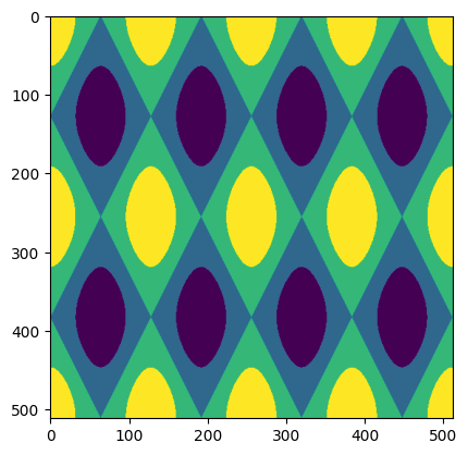
上图展示了我们的网络将要学习的目标。 

网络

接下来，让我们定义一个简单的卷积神经网络。输入是一个二维“图像”，其中通道是给定位置的 (x, y) 坐标，输出是每个点上的正弦波的值。模型由一系列卷积层、批归一化和激活函数组成。

class ConvModel(torch.nn.Module):
    def __init__(self, hidden_size=256, n_hidden_layers=2):
        super().__init__()
        layers = [
            torch.nn.Conv2d(2, hidden_size, 1),
            torch.nn.BatchNorm2d(hidden_size),
            torch.nn.ReLU(),
        ]
        for i in range(n_hidden_layers):
            layers += [
                torch.nn.Conv2d(hidden_size, hidden_size, 1),
                torch.nn.BatchNorm2d(hidden_size),
                torch.nn.ReLU(),
            ]
        layers += [torch.nn.Conv2d(hidden_size, 1, 1)]
        self.model = torch.nn.Sequential(*layers)

    def forward(self, x):
        return self.model(x)

现在，让我们比较使用标准训练和启用 AMP（自动混合精度）训练时的训练时间和内存使用情况。 

标准训练循环

首先，我们定义一个“标准”训练循环。我们初始化我们的模型、损失函数和优化器，然后执行一个标准的循环 n_epochs（为简化起见，epoch 只是一个单一示例）。

def test_standard_training(n_epochs, inputs, targets, hidden_size, n_hidden_layers):
    """测试一个标准的训练循环"""
    model = ConvModel(hidden_size, n_hidden_layers).cuda()
    loss_fn = torch.nn.MSELoss()
    opt = torch.optim.Adam(model.parameters(), 0.001)

    with TorchMemProfile() as profile:
        for i in range(n_epochs):
            opt.zero_grad()

            outputs = model(inputs)
            loss = loss_fn(outputs, targets)
            loss.backward()
            opt.step()

    return profile, loss, outputs

AMP训练循环 

接下来，让我们定义一个包含自动混合精度（AMP）的训练循环。我们可以看到一些关键的区别（代码中有注释）：

• 我们实例化了一个 torch.cuda.amp.GradScaler，该工具将用于缩放梯度以防止溢出或下溢

• 我们将前向传播和损失计算包裹在 torch.autocast 中

注意：

我们*不会*将反向传播或优化器步操作包裹在 torch.autocast 中。这些步骤仍将在可能的情况下以较低精度运行，但在必要时会进行升级，例如更新权重时。

def test_amp_training(n_epochs, inputs, targets, hidden_size, n_hidden_layers):
    """包含自动混合精度的训练循环"""
    model = ConvModel(hidden_size, n_hidden_layers).cuda()
    loss_fn = torch.nn.MSELoss()
    opt = torch.optim.Adam(model.parameters(), 0.001)

    scaler = torch.cuda.amp.GradScaler()             # 创建梯度缩放器

    with TorchMemProfile() as profile:
        for i in range(n_epochs):
            opt.zero_grad()
            with torch.autocast(device_type="cuda"):  # 仅将前向传播和损失计算包裹在 autocast 中
                outputs = model(inputs)
                loss = loss_fn(outputs, targets)
            scaler.scale(loss).backward()             # 对损失进行缩放，然后调用 backward
            scaler.step(opt)                          # 使用缩放器进行优化器的一步
            scaler.update()                           # 额外调用更新缩放器

    return profile, loss, outputs

标准训练与 AMP 性能比较

最后，让我们测试标准训练循环 vs AMP训练循环的相对性能。

# 定义训练参数
n_epochs = 512
hidden_size = 256
n_hidden_layers = 2

# 运行标准训练
profile, loss, outputs = test_standard_training(n_epochs, inputs, targets, hidden_size, n_hidden_layers)

# 运行AMP训练
profile_amp, loss_amp, outputs_amp = test_amp_training(n_epochs, inputs, targets, hidden_size, n_hidden_layers)

print("Standard training:")
print(f"  Total time: {profile.duration:0.4f}s")
print(f"  Loss: {loss:0.4g}")
print(f"  Max memory allocated: {profile.max_memory_allocated/1024**2:0.4g} MB")

print("\nAMP training:")
print(f"  Total time: {profile_amp.duration:0.4f}s")
print(f"  Loss: {loss_amp:0.4g}")
print(f"  Max memory allocated: {profile_amp.max_memory_allocated/1024**2:0.4g} MB")

print(f"\nTraining speedup: {(1-profile_amp.duration/profile.duration)*100:0.2f}%")
print(f"Memory savings: {(1-profile_amp.max_memory_allocated/profile.max_memory_allocated)*100:0.2f}%")

Standard training:
Total time: 13.9817s
Loss: 0.01
Max memory allocated: 2061 KB

AMP training:
Total time: 7.4969s
Loss: 0.008296
Max memory allocated: 1035 KB

Training speedup: 46.38%
Memory savings: 49.79%

通过AMP训练可以显著提高训练速度（提高46%）并减少近50%的内存使用! 而且，我们的AMP启用的训练并没有性能损失，反而导致了稍微更低的损失。

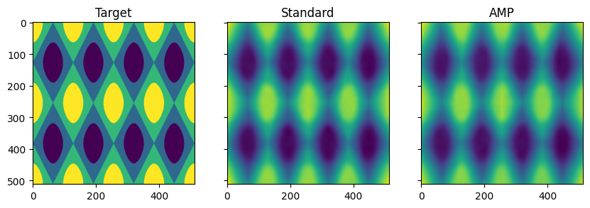
我们还可以通过可视化模型的输出来检查它们是否按照预期学习。我们看到标准训练和AMP训练都成功地逼近了我们的离散化2D正弦波。

fig, ax = plt.subplots(1, 3, sharex=True, sharey=True, figsize=(10, 4))
ax[0].imshow(targets.squeeze().cpu())
ax[1].imshow(outputs.squeeze().detach().cpu())
ax[2].imshow(outputs_amp.squeeze().detach().cpu())
ax[0].set_title("Target")
ax[1].set_title("Standard")
ax[2].set_title("AMP")
plt.show()

具有自动混合精度的推断

我们还可以通过将推理的前向传播过程包装起来以使用 AMP（自动混合精度）来加速推理。

为了演示这一点，我们将定义标准和 AMP 推理函数。请注意，对于 AMP 推理，我们不需要 GradScaler（因为没有梯度！），我们只需要将前向传播过程包装在 torch.autocast 中：

def test_standard_inference(n_epochs, inputs, hidden_size, n_hidden_layers):
    """测试标准训练循环"""
    model = ConvModel(hidden_size, n_hidden_layers).cuda()
    model.eval()

    with TorchMemProfile() as profile:
        for i in range(n_epochs):
            outputs = model(inputs)

    return profile


def test_amp_inference(n_epochs, inputs, hidden_size, n_hidden_layers):
    """测试标准训练循环"""
    model = ConvModel(hidden_size, n_hidden_layers).cuda()
    model.eval()

    with TorchMemProfile() as profile:
        for i in range(n_epochs):
            with torch.autocast(device_type="cuda"):
                outputs = model(inputs)

    return profile

# 运行标准推理
inf_profile = test_standard_inference(n_epochs, inputs, hidden_size, n_hidden_layers)

# 运行 AMP 推理
inf_profile_amp = test_amp_inference(n_epochs, inputs, hidden_size, n_hidden_layers)

print("Standard inference:")
print(f"  Total time: {inf_profile.duration:0.4f}s")
print(f"  Max memory allocated: {inf_profile.max_memory_allocated/1024**2:0.4g} MB")

print("\nAMP inference:")
print(f"  Total time: {inf_profile_amp.duration:0.4f}s")
print(f"  Max memory allocated: {inf_profile_amp.max_memory_allocated/1024**2:0.4g} MB")

print(f"\nSpeedup: {(1-inf_profile_amp.duration/inf_profile.duration)*100:0.2f}%")
print(f"Memory savings: {(1-inf_profile_amp.max_memory_allocated/inf_profile.max_memory_allocated)*100:0.2f}%")

输出结果如下：

Standard inference:
    Total time: 4.2401s
    Max memory allocated: 3338 MB

AMP inference:
    Total time: 2.8737s
    Max memory allocated: 1676 MB

Speedup: 32.23%
Memory savings: 49.79%

我们再次看到最大内存使用量减少了近 50%。然而，在推理过程中加速仅为 32%，相比训练过程中观察到的 46%。这种差异是因为部分加速是在反向传播过程中实现的，而推理时不涉及反向传播。

附录

运行在本地主机

如果您不想使用 Docker，您也可以直接在本地计算机上运行本文中的代码 - 虽然这样做需要一些额外的工作。

• 先决条件:

  • 安装ROCm 6.0.x

  • 确保您已安装 Python 3.11

  • 安装 PDM - 用于创建可复现的 Python 环境

• 在本博客的根目录中创建 Python 虚拟环境，并安装所有依赖项：

  pdm sync
  

• 启动 notebook

  pdm run jupyter-lab
  

导航到https://localhost:8888并运行本博客.