初始化
模型定义,初始化。Model的__init__函数:
class Model(nn.Module):
    r"""Spatial temporal graph convolutional networks.

    Args:
        in_channels (int): Number of channels in the input data
        num_class (int): Number of classes for the classification task
        graph_args (dict): The arguments for building the graph
        edge_importance_weighting (bool): If ``True``, adds a learnable
            importance weighting to the edges of the graph
        **kwargs (optional): Other parameters for graph convolution units

    Shape:
        - Input: :math:`(N, in_channels, T_{in}, V_{in}, M_{in})`
        - Output: :math:`(N, num_class)` where
            :math:`N` is a batch size,
            :math:`T_{in}` is a length of input sequence,
            :math:`V_{in}` is the number of graph nodes,
            :math:`M_{in}` is the number of instance in a frame.
    """

    def __init__(self, in_channels, num_class, graph_args,
                 edge_importance_weighting, **kwargs):
        super().__init__()

        # load graph
        self.graph = Graph(**graph_args)
        A = torch.tensor(self.graph.A, dtype=torch.float32, requires_grad=False)
        self.register_buffer('A', A)

        # build networks
        spatial_kernel_size = A.size(0)
        temporal_kernel_size = 9
        kernel_size = (temporal_kernel_size, spatial_kernel_size)
        self.data_bn = nn.BatchNorm1d(in_channels * A.size(1))
        kwargs0 = {k: v for k, v in kwargs.items() if k != 'dropout'}
        self.st_gcn_networks = nn.ModuleList((
            st_gcn(in_channels, 64, kernel_size, 1, residual=False, **kwargs0),
            st_gcn(64, 64, kernel_size, 1, **kwargs),
            st_gcn(64, 64, kernel_size, 1, **kwargs),
            st_gcn(64, 64, kernel_size, 1, **kwargs),
            st_gcn(64, 128, kernel_size, 2, **kwargs),
            st_gcn(128, 128, kernel_size, 1, **kwargs),
            st_gcn(128, 128, kernel_size, 1, **kwargs),
            st_gcn(128, 256, kernel_size, 2, **kwargs),
            st_gcn(256, 256, kernel_size, 1, **kwargs),
            st_gcn(256, 256, kernel_size, 1, **kwargs),
        ))

        # initialize parameters for edge importance weighting
        if edge_importance_weighting:
            self.edge_importance = nn.ParameterList([
                nn.Parameter(torch.ones(self.A.size()))
                for i in self.st_gcn_networks
            ])
        else:
            self.edge_importance = [1] * len(self.st_gcn_networks)

        # fcn for prediction
        self.fcn = nn.Conv2d(256, num_class, kernel_size=1)
首先是建立邻接矩阵A:
# load graph
self.graph = Graph(**graph_args)
A = torch.tensor(self.graph.A, dtype=torch.float32, requires_grad=False)
self.register_buffer('A', A)
图卷积的kernel的大小决定分组数量的多少,因为kernel的权重是和这一组的节点相乘然后取平均,最后所有组的结果再相加。
A的形状是K*V*V,K是kernel_size(和论文里的partitioning method选取有关,uni-label是1,distance是2,spatial是3),默认是spatial,所以A是3*25*25的大小。他代表在每一组里面节点的相连关系。
具体构建方法在Graph类的get_adjacency函数:
    def get_adjacency(self, strategy):
        valid_hop = range(0, self.max_hop + 1, self.dilation)
        adjacency = np.zeros((self.num_node, self.num_node))
        for hop in valid_hop:
            adjacency[self.hop_dis == hop] = 1
        normalize_adjacency = normalize_digraph(adjacency)

        if strategy == 'uniform':
            A = np.zeros((1, self.num_node, self.num_node))
            A[0] = normalize_adjacency
            self.A = A
        elif strategy == 'distance':
            A = np.zeros((len(valid_hop), self.num_node, self.num_node))
            for i, hop in enumerate(valid_hop):
                A[i][self.hop_dis == hop] = normalize_adjacency[self.hop_dis ==
                                                                hop]
            self.A = A
        elif strategy == 'spatial':
            A = []
            for hop in valid_hop:
                a_root = np.zeros((self.num_node, self.num_node))
                a_close = np.zeros((self.num_node, self.num_node))
                a_further = np.zeros((self.num_node, self.num_node))
                for i in range(self.num_node):
                    for j in range(self.num_node):
                        if self.hop_dis[j, i] == hop:
                            if self.hop_dis[j, self.center] == self.hop_dis[
                                    i, self.center]:
                                a_root[j, i] = normalize_adjacency[j, i]
                            elif self.hop_dis[j, self.
                                              center] > self.hop_dis[i, self.
                                                                     center]:
                                a_close[j, i] = normalize_adjacency[j, i]
                            else:
                                a_further[j, i] = normalize_adjacency[j, i]
                if hop == 0:
                    A.append(a_root)
                else:
                    A.append(a_root + a_close)
                    A.append(a_further)
            A = np.stack(A)
            self.A = A
        else:
            raise ValueError("Do Not Exist This Strategy")
要注意A是有一个normalize操作的,比如一个节点在这一组里相连的节点有2个
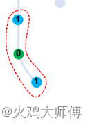
那这两个节点的数值都是1/2,对应文章里的这个部分
然后是初始化gcn网络模块,edge importance 权重参数,和最后的分类器
前向传播
def forward(self, x):

    # data normalization
    N, C, T, V, M = x.size()
    x = x.permute(0, 4, 3, 1, 2).contiguous()
    x = x.view(N * M, V * C, T)
    x = self.data_bn(x)
    x = x.view(N, M, V, C, T)
    x = x.permute(0, 1, 3, 4, 2).contiguous()
    x = x.view(N * M, C, T, V)

    # forwad
    for gcn, importance in zip(self.st_gcn_networks, self.edge_importance):
        x, _ = gcn(x, self.A * importance)

    # global pooling
    x = F.avg_pool2d(x, x.size()[2:])
    x = x.view(N, M, -1, 1, 1).mean(dim=1)

    # prediction
    x = self.fcn(x)
    x = x.view(x.size(0), -1)

    return x
我们先来看输入数据及其存储方式,输入数据的维度是(N,C,T,V,M),其中N是batch,C是channel,T是时间,V是节点,M是instance(例如一个时间输入可能包含两个骨架)
数据首先经过一系列reshape和Batch Normalization之后,输入gcn模块,这时候数据形状为(N*M,C,T,V)
st-gcn一共有10层gcn,其中第一层没有dropout,其余都有。
gcn内部
def forward(self, x, A):

    res = self.residual(x)
    x, A = self.gcn(x, A)
    x = self.tcn(x) + res

    return self.relu(x), A
x先是通过一个residual模块,本质是一个1x1卷积
self.residual = nn.Sequential(
    nn.Conv2d(
        in_channels,
        out_channels,
        kernel_size=1,
        stride=(stride, 1)),
    nn.BatchNorm2d(out_channels),
)
时空图卷积被分为空间卷积(spatial convolution)和时间卷积(temporal convolution)两个步骤来完成,在进行时间卷积时,可以直接调用1d卷积,因为时间上的相邻关系在矩阵中自然体现的,但是在空间卷积中,矩阵中节点并不是按相邻关系排布的,需要额外考虑邻接矩阵。
首先是空间卷积,x和A被输入空间卷积模块gcn中
self.gcn = ConvTemporalGraphical(in_channels, out_channels,
                                    kernel_size[1])
def forward(self, x, A):
assert A.size(0) == self.kernel_size
x = self.conv(x)
n, kc, t, v = x.size()
x = x.view(n, self.kernel_size, kc//self.kernel_size, t, v)
x = torch.einsum('nkctv,kvw->nctw', (x, A))
return x.contiguous(), A其本质也是用卷积实现的
self.conv = nn.Conv2d(
    in_channels,
    out_channels * kernel_size,
    kernel_size=(t_kernel_size, 1),
    padding=(t_padding, 0),
    stride=(t_stride, 1),
    dilation=(t_dilation, 1),
    bias=bias)
在实现spatial convolution时,为了考虑节点与卷积核计算的连接关系,将乘法和加法分开运算了,按理说应该是 out_channel 个 1x3 的卷积核,输出 out_channel 维度的特征,但是因为数据在矩阵中的存储方式,相邻节点并不一定有相邻关系,所以不能直接用2d卷积核运算。
这个地方,作者是采用 3*out_channel 个1x1 卷积核,这一步相当于是在做乘法运算(假定所有节点相连,所以会有计算冗余),输出 3*out_channel 维度的特征,维度是(N,K*C,T,V)然后reshape成(N,K,C,T,V)。
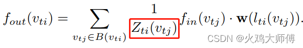
einsum这个函数是用来做加法操作。对每一个样本(N,T),模型的输出矩阵(K,V,C)需要与邻接矩阵A(K,V,W)做element-wise乘加,对于每一个节点W,他的相邻关系是一个矩阵(K,V),他的卷积核乘法输出是矩阵(K,V,C),这两个矩阵做element-wise相乘,最后再求和得到最终的输出向量(长度为C),就得到了这一个节点通过空间卷积核的输出(N,C,T,W)
然后时间卷积是一个普通的1d卷积核
self.tcn = nn.Sequential(
    nn.BatchNorm2d(out_channels),
    nn.ReLU(inplace=True),
    nn.Conv2d(
        out_channels,
        out_channels,
        (kernel_size[0], 1),
        (stride, 1),
        padding,
    ),
    nn.BatchNorm2d(out_channels),
    nn.Dropout(dropout, inplace=True),
)
空间卷积的输出经过时间卷积之后,加上残差模块的输出,就得到了gcn模块的输出,这样的gcn模块一共有十个。
def forward(self, x, A):

    res = self.residual(x)
    x, A = self.gcn(x, A)
    x = self.tcn(x) + res

    return self.relu(x), A
然后是一个global pooling层,将T*V的feature聚合到一个特征向量,再reshape回(N,M,C,1,1),然后跨instance取平均,得到(N,C,1,1)
# global pooling
x = F.avg_pool2d(x, x.size()[2:])
x = x.view(N, M, -1, 1, 1).mean(dim=1)

# prediction
x = self.fcn(x)
x = x.view(x.size(0), -1)
最后是一个卷积神经网络(1x1卷积核作用于1x1的图,其实相当于全连接)输出类别向量
# fcn for prediction
self.fcn = nn.Conv2d(256, num_class, kernel_size=1)