PINNs案例——中心热源温度场预测问题的torch代码

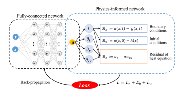
基于物理信息的神经网络（Physics-Informed Neural Networks，PINNs）作为一种新兴的机器学习框架，为解决偏微分方程（Partial Differential Equations，PDEs）计算问题提供了全新的思路和途径。其核心思想是将神经网络与物理定律相结合，通过将 PDEs 作为网络训练过程中的约束条件，使得神经网络能够在学习数据的同时，也满足物理定律的约束。

PINN网络结构示意图

今天来分享博主自己复现的一个简单的PINNs代码实现案例：中心热源温度场预测

该案例参考学习论文：[1]陆至彬,瞿景辉,刘桦等.基于物理信息神经网络的传热过程物理场代理模型的构建[J].化工学报,2021,72(03):1496-1503.

PINN求解结果

catalogue

问题场景

**求解域：**案例选取边长为 1 的正方形区域作为研究对象，即定义域为
$\Omega = [-0.5, 0.5] \times [-0.5, 0.5]$ 。以正方形中心为原点，且原点处为热源。
**参数设定：**热源处 $q = 1$ ，材料热导率在{ κ ∈ R:0.5 ≤ κ ≤ 1}}内变化。热导率满足参数θ，相应的参数θ变化范围为{θ = q/κ ∈ R:1 ≤ θ ≤ 2}。
**边界条件：**方形四周的边界温度恒为1
**求解量：**区域内二维稳态温度场分布

PINNs理论求解

在该正方形区域内，温度场 $ T(x, y) $ 满足二维稳态导热方程，数学表达为：
$-\kappa \left( \frac{\partial^2 T}{\partial x^2} + \frac{\partial^2 T}{\partial y^2} \right) = q$

其中：

$\kappa$ 为材料的热导率（thermal conductivity），表示材料传导热量的能力；
$q$ 为内热源（heat source），表示单位体积内热量的产生率；
$T (x, y)$ 为温度分布函数。

PINNs 通过构建一个深度神经网络来近似温度场 $T (x, y)$ ，并通过优化损失函数来训练网络，使其输出同时满足控制方程和边界条件。神经网络框架能够利用自动微分计算偏导数，将物理约束嵌入神经网络的学习过程中。

损失函数通常包含两部分：

PDE 残差项：确保网络输出满足控制方程。根据案例控制方程：
$\text{Loss}_{\text{PDE}} = \frac{1}{N_c} \sum_{i=1}^{N_c} \left| f\left( x_c^i, y_c^i \right) \right|^2$
$f\left( x_c^i, y_c^i \right) = q -\kappa \left( \frac{\partial^2 T}{\partial x^2} + \frac{\partial^2 T}{\partial y^2} \right)$
边界条件项：确保网络输出在边界上的预测符合给定条件。该案例中可以使用两种边界条件形式：

软边界条件：软边界条件通过将边界约束作为损失函数的一部分来实现,其边界损失可以表示为：
$\text{Loss}_{\text{BC}} = \frac{1}{N_b} \sum_{i=1}^{N_b} \left| T\left( x_b^i, y_b^i \right) - 0 \right|^2$

这种方法通过最小化边界误差来近似满足边界 $T = 0$

硬边界条件：
硬边界条件通过网络结构的预设计，使输出自动满足边界条件。以该案例为例，可令网络输出温度：
$\cdot \hat{T}(x, y)$
其中：
$\hat{T}(x, y)$ 是神经网络的原始输出，
$D (x, y)$ 是一个辅助函数，定义为在边界上为零。对于本求解问题可选择：
$D(x, y) = (x^2-0.25)*(y^2 - 0.25)$
由于 $D (x, y)$ 在 $x = - 0.5, 0.5$ 或 $y = - 0.5, 0.5$ 时值为零，因此 $T (x, y)$ 自动满足边界条件 $T = 0$ 。
此时，损失函数仅需考虑 PDE 残差,硬边界条件通过结构设计确保边界条件的精确满足，减少了训练过程中对边界误差的优化需求，通常在边界附近表现更优。

$N_{bc}$ 表示边界上的取点数量， $N_{C}$ 表示内部需要满足对应控制方程的点

复现结果

软边界PINN结果

硬边界PINN结果

软边界损失函数

硬边界损失函数

pytorch代码

软边界：
导入相关包

import numpy as np
import matplotlib.pyplot as plt
import torch
import torch.nn as nn
from torch.autograd import grad
from pyDOE import lhs

import time

定义设备：

device = torch.device("cuda") if torch.cuda.is_available() else torch.device("cpu")

#设置区域范围
x_min = -0.5
x_max = 0.5
y_min = -0.5
y_max = 0.5

ub = np.array([x_max, y_max])
lb = np.array([x_min, y_min])

N_b = 4000   #垂直边界点数量
N_w = 4000   #水平边界点数量
N_c = 4000  #内点数量

# 定义温度常量

T_fixed = 1 # 边界温度
T_inf = 0    # 环境温度
T_max = 1
T_min = 0

q=1
k = q/1.5


#生成边界数据
    wall1_xy = [x_min, y_min] + [0, y_max-y_min] * lhs(2, N_b)  #x=0边界，   lhs(2, N_b)：生成一个 二维 采样点为N_b 的拉丁超立方采样矩阵     [x_min, y_min]， [0.0, y_max] 表示范围
    wall1_T = T_fixed * np.ones((N_b, 1))  #左边界固定温度


    wall2_xy = [x_max, y_min] + [0, y_max-y_min] * lhs(2, N_b)    #右边界环境温度
    wall2_T = T_fixed * np.ones((N_b, 1))

    wall3_xy = [x_min, y_max] + [x_max-x_min,0] * lhs(2, N_w)   #顶边界
    wall3_T = T_fixed * np.ones((N_w, 1))

    wall4_xy = [x_min, y_min] + [x_max-x_min, 0] * lhs(2, N_w)  #底边界固定温度
    wall4_T = T_fixed * np.ones((N_w, 1))

    xy_bnd = np.concatenate([wall1_xy, wall2_xy, wall3_xy, wall4_xy], axis=0)  #合并边界坐标
    T_bnd = np.concatenate([wall1_T, wall2_T, wall3_T, wall4_T], axis=0)   #合并边界温度
    T_bnd = (T_bnd - T_min) / (T_max - T_min)    #归一化

    xy_col = lb + (ub - lb) * lhs(2, N_c)  #内部点采样，lhs(2, N_c) 会返回一个 [N_c, 2] 的矩阵，其中的每一行表示一个在该范围内随机生成的坐标点。
    xy_all = np.concatenate((xy_col, xy_bnd), axis=0)  #合并边界和内部点

    xy_bnd = torch.tensor(xy_bnd, dtype=torch.float32).to(device)  #边界点
    T_bnd = torch.tensor(T_bnd, dtype=torch.float32).to(device)   #边界温度
    xy_col = torch.tensor(xy_col, dtype=torch.float32).to(device)   #内部采样点
    xy_all = torch.tensor(xy_all, dtype=torch.float32).to(device)   #内部采样点

    return xy_col, xy_bnd, T_bnd, xy_all

xy_col, xy_bnd, T_bnd , xy_all = getData()

定义网络结构：

# Learning process

def weights_init(m):
    if isinstance(m, nn.Linear):
        torch.nn.init.xavier_uniform_(m.weight.data)
        torch.nn.init.zeros_(m.bias.data)


class layer(nn.Module):

    def __init__(self, n_in, n_out, activation):
        super().__init__()
        self.layer = nn.Linear(n_in, n_out)
        self.activation = activation

    def forward(self, x):
        x = self.layer(x)
        if self.activation:
            x = self.activation(x)
        return x

class DNN(nn.Module):
    # dim_in 和 dim_out：分别为网络的输入和输出维度，n_layer 和 n_node：n_layer 表示隐藏层的数量， activation为激活函数，ub 和 lb：分别是区域的上界和下界，用于输入的归一化处理。
    def __init__(self, dim_in, dim_out, n_layer, n_node, ub, lb, activation = nn.GELU()):
        super().__init__()
        self.net = nn.ModuleList()
        self.net.append(layer(dim_in, n_node, activation))  #第一个输入层
        for _ in range(n_layer):
            self.net.append(layer(n_node, n_node, activation))
        self.net.append(layer(n_node, dim_out, activation=None))   #最后一个输出层
        # self.ub = torch.tensor(ub, dtype=torch.float).to(device)
        # self.lb = torch.tensor(lb, dtype=torch.float).to(device)
        self.net.apply(weights_init)  # weights_init 函数对网络的权重和偏置进行初始化（例如 Xavier 初始化），从而提供较好的初始收敛性。

    def forward(self, x):
        out = x
        for layer in self.net:
            out = layer(out)
        return out

class PINN:

    def __init__(self) -> None:
        self.net = DNN(dim_in=2, dim_out=1, n_layer=5, n_node=50, ub=ub, lb=lb).to(
            device
        )

        self.lbfgs = torch.optim.LBFGS(
            self.net.parameters(),
            lr=0.1,
            max_iter=20000,
            max_eval=20000,
            tolerance_grad=1e-5,
            tolerance_change= 1 * np.finfo(float).eps,
            history_size=50,
            line_search_fn="strong_wolfe",
        )

        #分别定义了 LBFGS 和 Adam 两种优化器。LBFGS 是一种基于二阶信息的优化算法，适用于物理信息神经网络的优化；Adam 是一种常用的一阶优化方法，用于更新网络权重。

        self.adam = torch.optim.Adam(self.net.parameters(), lr=1e-4)
        self.losses = {
    
    "bc": [], "pde": [],"loss": []}
        self.iter = 0

    def predict(self, xy):
        out = self.net(xy)
        # 反归一化
        # T = out * (T_max - T_min) + T_min
        T=out
        return T

边界条件损失函数：

    def bc_loss(self, xy):
       
        xy = xy.clone()
        xy.requires_grad = True  # 设置xy可求导
        #边界条件温度归一化
        T_inf_norm =(T_inf-T_min) / (T_max - T_min)
        T_fixed_norm =(T_fixed-T_min) / (T_max - T_min)

        # 预测温度
        T_bnd = self.predict(xy)
        # 边界条件处理
        l = torch.mean(torch.square(T_bnd - T_fixed_norm))
        mse_bc = l
        return mse_bc

PDE损失：

    def pde_loss(self, xy):
        xy = xy.clone()
        xy.requires_grad = True  #设置xy可求导

        T = self.predict(xy)

        T_out = grad(T.sum(), xy, create_graph=True)[0]  #一阶导数
        T_out2 = grad(T_out.sum(), xy, create_graph=True)[0] #二阶导数

        #偏导数
        T_x = T_out[:, 0:1]
        T_y = T_out[:, 1:2]
        T_xx = T_out2[:, 0:1]
        T_yy = T_out2[:, 1:2]

        f0 =k* (T_xx + T_yy) + q

        mse_f0 = torch.mean(torch.square(f0)) #元素平方和的平均

        mse_pde = mse_f0
        #微分方程损失
        return mse_pde

闭包函数：


    def closure(self):

        self.lbfgs.zero_grad()
        self.adam.zero_grad()

        mse_bc = self.bc_loss(xy_bnd)
        mse_pde = self.pde_loss(xy_col)

        loss = 5*mse_bc + mse_pde

        loss.backward()

        self.losses["bc"].append(mse_bc.detach().cpu().item())
        self.losses["pde"].append(mse_pde.detach().cpu().item())
        self.losses["loss"].append(loss.cpu().item())

        self.iter += 1

        print(
            f"\r It: {
      
      self.iter} Loss: {
      
      loss.item():.5e} BC: {
      
      mse_bc.item():.3e}  pde: {
      
      mse_pde.item():.3e}",
            end="",
        )

        if self.iter % 100 == 0:
            print("")

        return loss

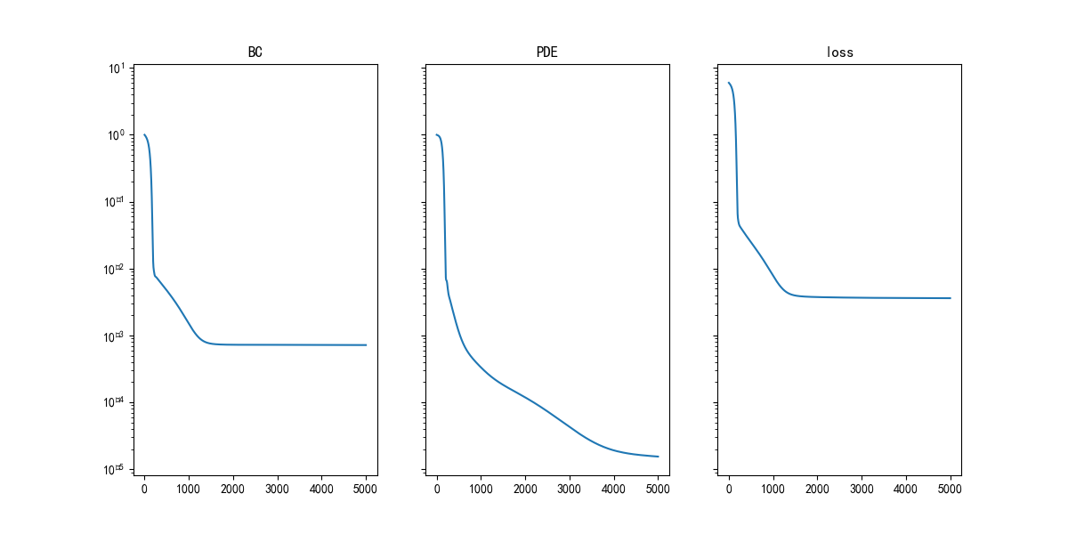
损失曲线保存：

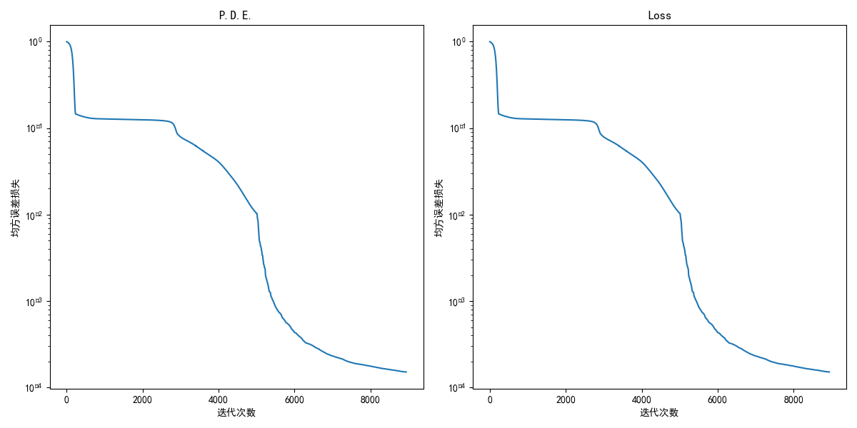
def plotLoss(losses_dict, path, info=["B.C.", "P.D.E.","Loss"]):
    fig, axes = plt.subplots(1, 3, sharex=True, sharey=True, figsize=(12, 6))
    axes[0].set_yscale("log")
    for i, j in zip(range(3), info):
        axes[i].plot(losses_dict[j.lower()])
        axes[i].set_title(j)
    plt.show()
    fig.savefig(path)

主函数：


if __name__ == "__main__":

    pinn = PINN()
    start_time = time.time()
    pointsplot()
    for i in range(5000):
        pinn.closure()
        pinn.adam.step()
    pinn.lbfgs.step(pinn.closure) #使用lbfgs优化器快速收敛，调整收敛结果，如需控制迭代次数可删除本行

    print("--- %s seconds ---" % (time.time() - start_time))
    print(f'-- {
      
      (time.time() - start_time)/60} mins --')
    torch.save(pinn.net.state_dict(), "Param.pt")
    plotLoss(pinn.losses, "LossCurve.png", ["BC", "PDE","loss"])

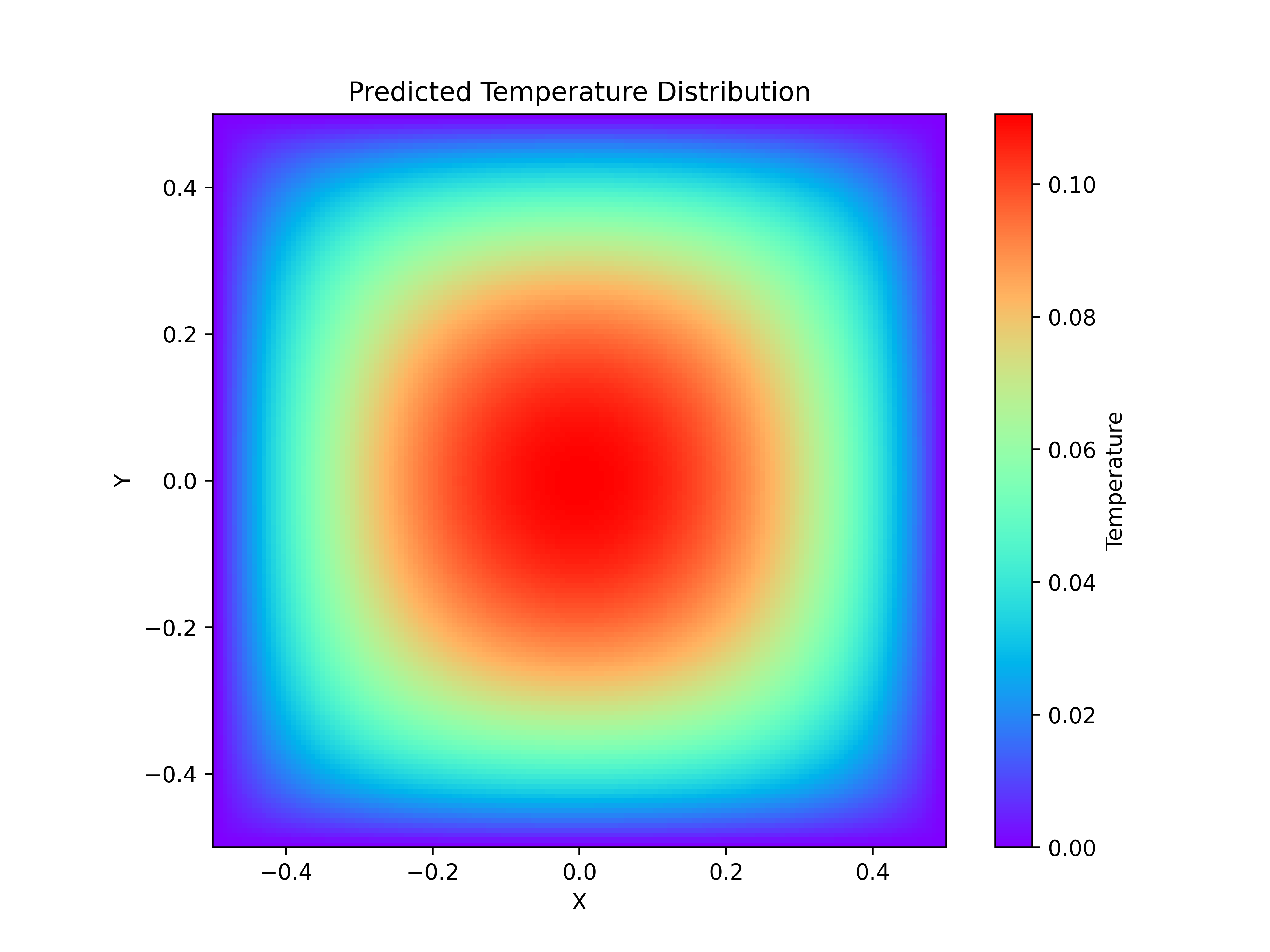
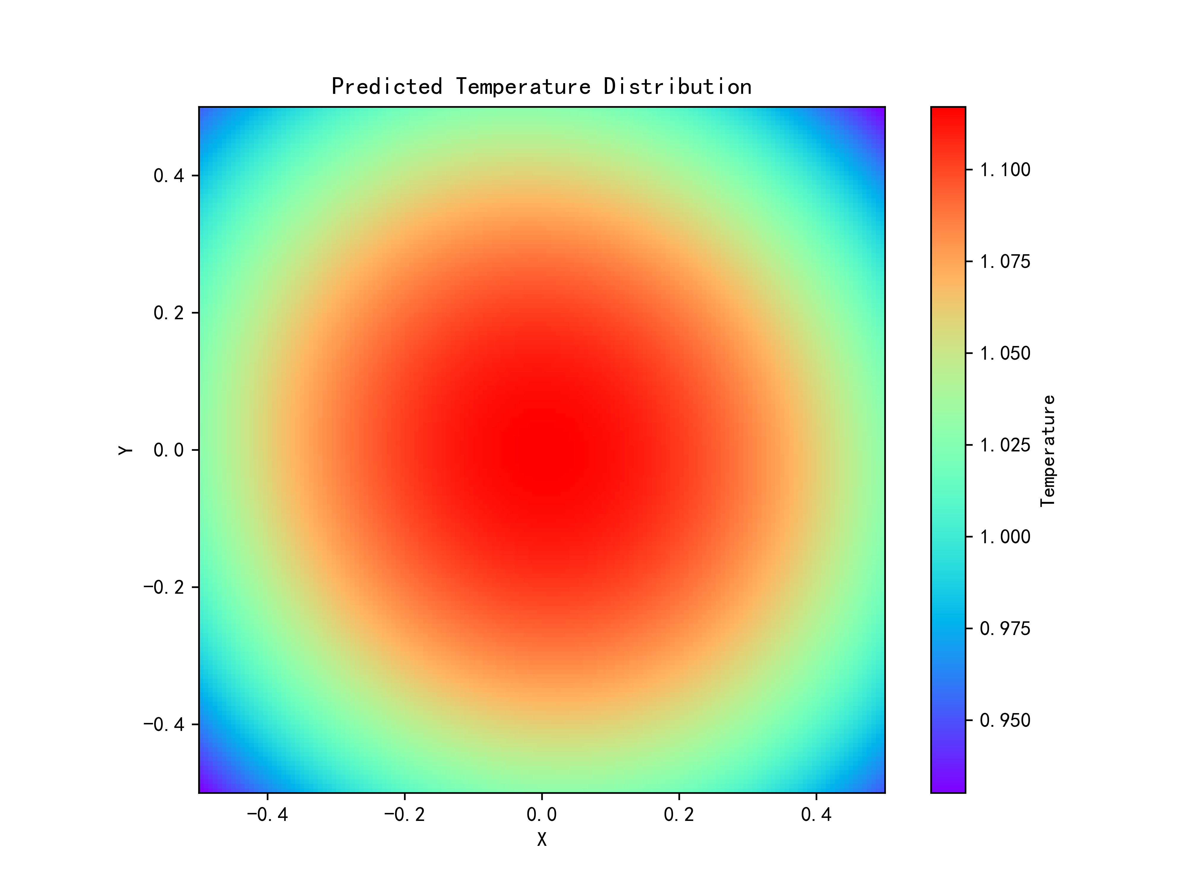
预测结果可视化eval.py

import numpy as np
import matplotlib.pyplot as plt
import torch
from main import PINN
from hardPINN import PINN as hardPINN


device = torch.device("cuda") if torch.cuda.is_available() else torch.device("cpu")
hard = True


# 定义网格的分辨率
grid_size_x = 150
grid_size_y = 150
x_min = -0.5
x_max = 0.5
y_min = -0.5
y_max = 0.5
T_max = 1
T_min = 0

# 生成x和y坐标的等距网格点
x = np.linspace(x_min, x_max, grid_size_x)
y = np.linspace(y_min, y_max, grid_size_y)
X, Y = np.meshgrid(x, y)

# 将网格点转化为输入格式（grid_size * grid_size, 2）
xy_grid = np.hstack((X.reshape(-1, 1), Y.reshape(-1, 1)))
xy_grid = torch.tensor(xy_grid, dtype=torch.float32).to(device)

if hard:
    pinn = hardPINN()
    pinn.net.load_state_dict(torch.load("ParamHard.pt"))
else:
    pinn = PINN()
    pinn.net.load_state_dict(torch.load("Param.pt"))

# 预测温度
with torch.no_grad():
    T_pred = pinn.predict(xy_grid)

# 将预测的温度值转化为numpy格式，并恢复为网格形状
T_pred = T_pred.cpu().numpy().reshape(Y.shape)
print(T_pred)
# T_pred =T_pred*(T_max-T_min)+T_min
print(T_pred.max())

plt.figure(figsize=(8, 6))
plt.imshow(T_pred, extent=(x_min, x_max, y_min, y_max), origin='lower', cmap='rainbow')
plt.colorbar(label='Temperature')
plt.xlabel('X')
plt.ylabel('Y')
plt.title('Predicted Temperature Distribution')
path = "solH.png" if hard else "sol.png"
plt.savefig(path, dpi=500)
plt.show()

完整代码及硬边界代码请关注小姜公众号获取。相关代码问题也可在Freshman小姜公众号咨询！

期待下一期PINNs案例代码分享吧！

catalogue

问题场景

PINNs理论求解

复现结果

pytorch代码

猜你喜欢

目录

热门文章