以区分手写数字5,8为例。

代码如下：

import cv2
import numpy as np
from matplotlib import pyplot as plt

def grid_feature(im,grid=(9,16)):
    gh=grid[0]
    gw=grid[1]
    h,w = im.shape
    _,im = cv2.threshold(im, 128, 255, cv2.THRESH_BINARY)
    sh = h // gh
    sw = w // gw
    gridFeat = np.zeros((gh*gw))
    for i in range(gh):
        for j in range(gw):
            tmp = im[sh * i:sh * (i+1) + 1, sw*j: sw * (j+1) +1]
            gridFeat[i * gw + j] = np.sum(tmp)
    gridFeat = gridFeat / (np.sum(gridFeat))
    return gridFeat

nGrids = [3, 3]
nDim = nGrids[0] * nGrids[1]
nTot = 50  # 数据集大小
nTrain = 40  # 训练集数量
nTest = nTot - nTrain

posTrainData = np.zeros(shape=(nTrain, nDim))
for i in range(1, nTrain + 1):
    im = cv2.imread("E:/data/5/{}.jpg".format(i), 0)
    aFeat = grid_feature(im, nGrids)
    posTrainData[i - 1] = aFeat

negTrainData = np.zeros(shape=(nTrain, nDim))
for i in range(1, nTrain + 1):
    im = cv2.imread("E:/data/8/{}.jpg".format(i), 0)
    aFeat = grid_feature(im, nGrids)
    negTrainData[i - 1] = aFeat

testData = np.zeros(shape=(nTest * 2, nDim))
for i in range(nTrain + 1, nTot + 1):
    im = cv2.imread("E:/data/5/{}.jpg".format(i), 0)
    aFeat = grid_feature(im, nGrids)
    testData[i - nTrain - 1] = aFeat
for i in range(nTrain + 1, nTot + 1):
    im = cv2.imread("E:/data/8/{}.jpg".format(i), 0)
    aFeat = grid_feature(im, nGrids)
    testData[nTest + i - nTrain - 1] = aFeat

# logistic回归
xTrain = np.concatenate((posTrainData, negTrainData))
yTrain = np.concatenate((np.ones(nTrain), np.zeros(nTrain))).reshape(-1, 1)
xTest = testData
yTest = np.concatenate((np.ones(nTest), np.zeros(nTest))).reshape(-1, 1)
omega = np.array(np.random.rand(nDim, 1) - np.random.rand(nDim, 1))

count = 0
maxIter = 1e5
cvgVal = 1e-7
allTrErr = np.array([])
allTsErr = np.array([])
allLoss = np.array([])

alpha = 0.1  # 学习率
sigmoid = lambda x: 1 / (1 + np.exp(-1 * x))

# 1 当前omega下训练样本的决策函数值
yTrRs = sigmoid(np.matmul(xTrain, omega))  # 80*1
# 2 当前omega下损失函数值
loss0 = -1 * np.mean(yTrain * np.log(yTrRs) + (1 - yTrain) * np.log(1 - yTrRs))

while count < maxIter:
    count += 1
    allLoss = np.append(allLoss, loss0)
    deltaY = yTrain - yTrRs
    # 3 求梯度，反方向即为omega更新方向
    directOmega = np.matmul(xTrain.T, deltaY)  # 9*1 #梯度更新方向
    # 4 更新omega
    omega = omega + alpha * directOmega
    # 5 新omgea下训练样本的决策函数值
    yTrRs = sigmoid(np.matmul(xTrain, omega))
    # 6 新omgea下损失函数值
    loss1 = -1 * np.mean(yTrain * np.log(yTrRs) + (1 - yTrain) * np.log(1 - yTrRs))
    # 损失函数值的下降率
    deltaLoss = loss0 - loss1
    lossRate = deltaLoss / loss0
    # 7 训练样本的预测标签
    yTrLabel = np.array([1 if x > 0.5 else 0 for x in yTrRs]).reshape(-1, 1)
    trErr = 1 - np.mean(yTrLabel == yTrain)
    allTrErr = np.append(allTrErr, trErr)
    # 8 测试样本的预测标签
    yPred = sigmoid(np.matmul(xTest, omega))
    yPredLabel = np.array([1 if x > 0.5 else 0 for x in yPred]).reshape(-1, 1)
    tsErr = 1 - np.mean(yPredLabel == yTest)
    allTsErr = np.append(allTsErr, tsErr)
    if count % 100 == 0:
        print("iter:{}, alpha: {:.1f}, loss: {:.3e}, dscRate: {:.1e}, TrErr: {:.4f}, TsErr: {:.4f}".format(count, alpha, loss1,
                                                                                                      lossRate, trErr, tsErr))
    # 下降率是否达到预设值
    if 0 <= lossRate < cvgVal:
        break
    loss0 = loss1

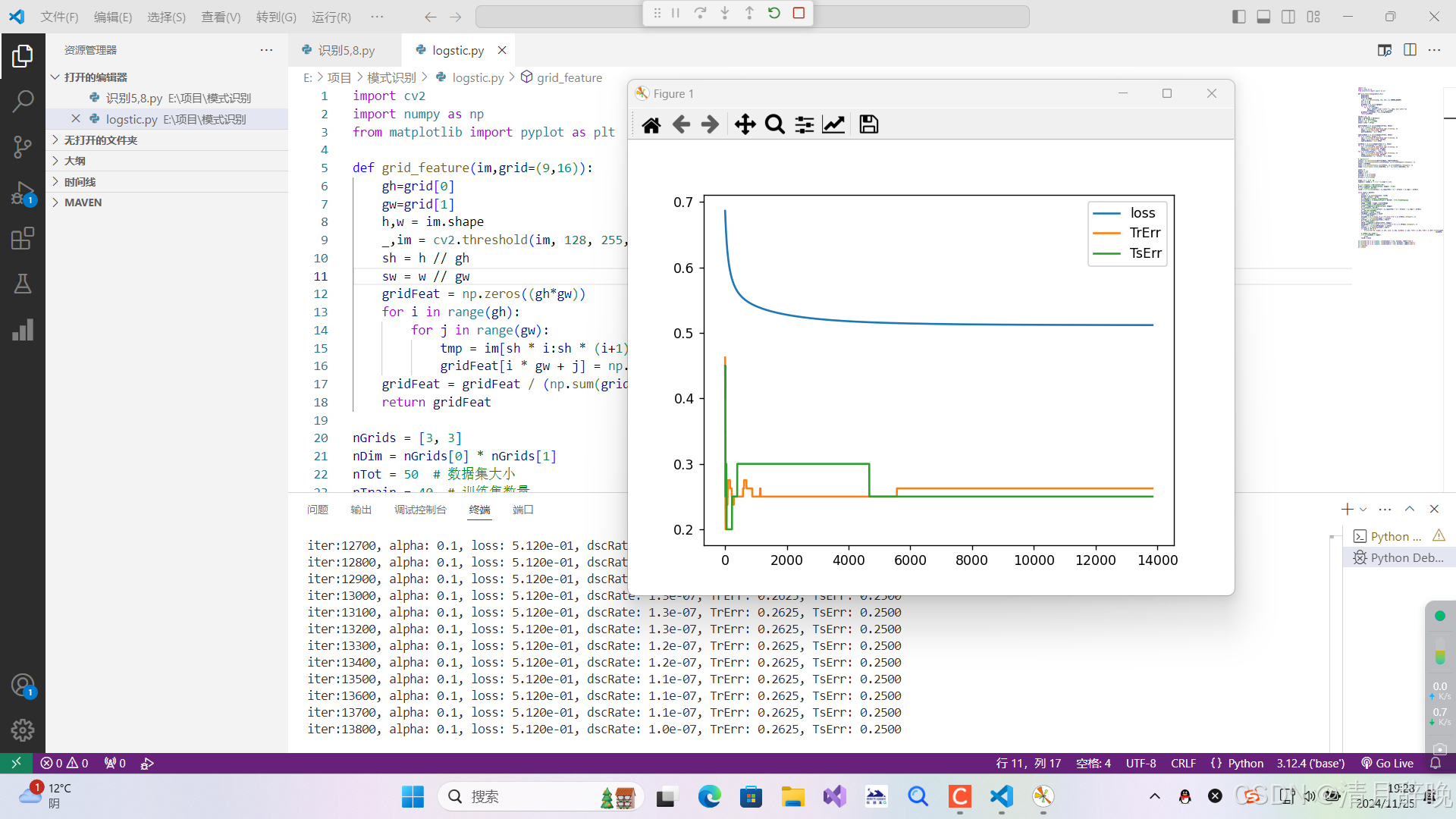
plt.plot([i for i in range(1, len(allLoss) + 1)], allLoss, label='loss')
plt.plot([i for i in range(1, len(allTrErr) + 1)], allTrErr, label='TrErr')
plt.plot([i for i in range(1, len(allTsErr) + 1)], allTsErr, label="TsErr")
plt.legend()
plt.show()

结果如下：