【1】引言

python具备强大的数据处理功能，但数据处理往往需要结合智能算法，本次文章就学习用python仿真模拟退火算法。

【2】模拟退火算法

模拟退火算法本质和其名称一样，以金属材料热处理的退火过程为模拟对象，模拟退火过程中的物理变化规律来处理数据。

当温度较高时，金属材料内的粒子具有较高的自由运动能量；随着温度降低，粒子的自由运动能量逐渐降低；完全冷却后，粒子没有自由运动能量，材料的性能达到稳定。

把这个过程映射到算法上，就是：

在自变量取极大值的时候，会获得对应因变量的值——高温状态，较高的粒子自由运动能量；

改变自变量，因变量的值变化，如果新的因变量小于初始变量，这个变化趋势就是可取的，否则新因变量的取值只能以概率的形式接受——温度降低，粒子自由运动能量跟随降低；

按照这个判断标准，因变量继续减小，直至准确判定因变量已经达到稳定值——完全冷却，粒子自由运动能量为0。

【3】代码实现

为在代码上实现这个过程，需要进一步细化。

【3.1】准备工作

首先引入必要的模块：

import numpy as np #引入numpy模块
import matplotlib.pyplot as plt #引入matplotlib模块

然后定义一个目标函数：

# 定义目标函数，这里是 f(x) = x^2
def objective_function(x):
    return x ** 2

这个目标函数就可以理解为粒子的自由运动能量。

之后定义一些初始变量：

# 初始化参数
# 初始解
initial_solution = np.random.uniform(-10, 20)
# 初始温度
initial_temperature = 100
# 终止温度
final_temperature = 0.01
# 温度衰减系数
alpha = 0.95
# 每个温度下的迭代次数
num_iterations_per_temp = 100

在这里，各个参数的意义是：

• 预设的初始能量：初始解 initial_solution = np.random.uniform(-10, 20) 
• 初始温度： 初始温度 initial_temperature = 100 
• 冷却温度： 终止温度 final_temperature = 0.01 
• 温度衰减系数： 温度衰减系数 alpha = 0.95 
• 每个温度下，往周围区域探索的次数： 每个温度下的迭代次数 num_iterations_per_temp = 100 

综合理解起来就是，温度逐渐降低，在每个温度附件，都要计算100次。

【3.2】模拟退火算法函数

定义模拟退火算法函数：

# 模拟退火算法
def simulated_annealing(initial_solution, initial_temperature, final_temperature, alpha, num_iterations_per_temp):
    # 当前解
    current_solution = initial_solution
    # 当前解的目标函数值
    current_energy = objective_function(current_solution)
    # 最优解
    best_solution = current_solution
    # 最优解的目标函数值
    best_energy = current_energy
    # 当前温度
    temperature = initial_temperature

    # 用于记录每一步的最优目标函数值
    energy_history = [best_energy]

    while temperature > final_temperature:
        for _ in range(num_iterations_per_temp):
            # 在当前解的邻域内生成新解
            new_solution = current_solution + np.random.uniform(-0.1, 0.1)
            # 计算新解的目标函数值
            new_energy = objective_function(new_solution)
            # 计算能量差
            delta_energy = new_energy - current_energy

            # 如果新解更优，直接接受
            if delta_energy < 0:
                current_solution = new_solution
                current_energy = new_energy
                # 更新最优解
                if new_energy < best_energy:
                    best_solution = new_solution
                    best_energy = new_energy
            # 如果新解更差，以一定概率接受
            else:
                acceptance_probability = np.exp(-delta_energy / temperature)
                if np.random.rand() < acceptance_probability:
                    current_solution = new_solution
                    current_energy = new_energy

            # 记录当前最优目标函数值
            energy_history.append(best_energy)

        # 降低温度
        temperature *= alpha

    return best_solution, best_energy, energy_history

这个自定义函数非常长，这里逐步分析：

def simulated_annealing(initial_solution, initial_temperature, final_temperature, alpha, num_iterations_per_temp):
    # 当前解
    current_solution = initial_solution
    # 当前解的目标函数值
    current_energy = objective_function(current_solution)
    # 最优解
    best_solution = current_solution
    # 最优解的目标函数值
    best_energy = current_energy
    # 当前温度
    temperature = initial_temperature

    # 用于记录每一步的最优目标函数值
    energy_history = [best_energy]

def simulated_annealing()函数需要一系列参数，这些参数被直接赋值：

current_solution是def simulated_annealing()函数自定义的参数，它的第一个值是提前定义好的initial_solution；

current_energy是def simulated_annealing()函数自定义的参数，它的取值是以current_solution为自变量，代入目标函数获得的；

best_solution 是def simulated_annealing()函数自定义的参数，它的第一个值是已经获得initial_solution赋值的current_solution；

best_energy 是def simulated_annealing()函数自定义的参数，它的第一个值是已经计算获得的current_energy；

temperature 是def simulated_annealing()函数自定义的参数，它的第一个值是提前定义好的initial_temperature；

此外有一个energy_history = [best_energy]，以列表的形似存储每一个best_energy。

到这里，其实完成了这些函数的第一个值定义。

然后要开始循环确认：

while temperature > final_temperature:
    for _ in range(num_iterations_per_temp):
        # 在当前解的邻域内生成新解
        new_solution = current_solution + np.random.uniform(-0.1, 0.1)
        # 计算新解的目标函数值
        new_energy = objective_function(new_solution)
        # 计算能量差
        delta_energy = new_energy - current_energy

        # 如果新解更优，直接接受
        if delta_energy < 0:
            current_solution = new_solution
            current_energy = new_energy
            # 更新最优解
            if new_energy < best_energy:
                best_solution = new_solution
                best_energy = new_energy
        # 如果新解更差，以一定概率接受
        else:
            acceptance_probability = np.exp(-delta_energy / temperature)
            if np.random.rand() < acceptance_probability:
                current_solution = new_solution
                current_energy = new_energy

        # 记录当前最优目标函数值
        energy_history.append(best_energy)

    # 降低温度
    temperature *= alpha

return best_solution, best_energy, energy_history

其中的第一部分：

for _ in range(num_iterations_per_temp):
    # 在当前解的邻域内生成新解
    new_solution = current_solution + np.random.uniform(-0.1, 0.1)
    # 计算新解的目标函数值
    new_energy = objective_function(new_solution)
    # 计算能量差
    delta_energy = new_energy - current_energy

这个for循环之内，_代表多次执行，_记录执行次数。

在这个for循环之内，具体的：

new_solution = current_solution + np.random.uniform(-0.1, 0.1)表示new_solution的取值，是用current_solution叠加一个位于(-0.1,0.1)之间的随机数，也就是new_solution是在current_solution的基础上进行微小变化；

new_energy = objective_function(new_solution)表示，使用获得的new_solution代入目标函数，获得新的因变量值；

delta_energy = new_energy - current_energy表示，新的因变量值减去上一步的因变量值。

在上述计算之后，到了条件判断过程：

# 如果新解更优，直接接受
if delta_energy < 0:
    current_solution = new_solution
    current_energy = new_energy
    # 更新最优解
    if new_energy < best_energy:
        best_solution = new_solution
        best_energy = new_energy
# 如果新解更差，以一定概率接受
else:
    acceptance_probability = np.exp(-delta_energy / temperature)
    if np.random.rand() < acceptance_probability:
        current_solution = new_solution
        current_energy = new_energy

首先，看上一步的计算结果delta_energy < 0是否成立，如果成立，会直接选用最新计算的结果：

current_solution = new_solution 

current_energy = new_energy

然后，在此基础上继续判断，如果new_energy < best_energy最新计算结果小于先前获得的最佳计算结果，就会将最新计算结果定义为最佳计算结果：

best_solution = new_solution 

best_energy = new_energy

需要注意的是，只有delta_energy < 0成立，才会继续判断new_energy < best_energy是否成立。

当delta_energy < 0不成立，此时的执行方式是：

先定义一个接受概率：acceptance_probability = np.exp(-delta_energy / temperature)

然后判断np.random.rand() < acceptance_probability是否成立，np.random.rand()代表生成一个在区间[0,1)均匀分布的随机数，因为概率的范围是[0,1]，所以np.random.rand()函数能和概率acceptance_probability来做对比。

当np.random.rand() < acceptance_probability成立，只接受最新值，不将最新值取为最佳值：

current_solution = new_solution 

current_energy = new_energy

然后需要在energy_history添加最新的best_energy。

# 记录当前最优目标函数值
energy_history.append(best_energy)

算完一个温度，需要降低温度继续计算，这时候就要用到：

# 降低温度
temperature *= alpha 

循环运算结束后，需要输出参数：

return best_solution, best_energy, energy_history

【3.3】输出计算结果

之后比较简单，直接运行代码，获得模拟退火运算的结果：

# 运行模拟退火算法
best_solution, best_energy, energy_history = simulated_annealing(initial_solution, initial_temperature, final_temperature, alpha, num_iterations_per_temp)

print("最优解:", best_solution)
print("最优值:", best_energy)

 综合起来，给出完整代码：

import numpy as np #引入numpy模块
import matplotlib.pyplot as plt #引入matplotlib模块

# 定义目标函数，这里是 f(x) = x^2
def objective_function(x):
    return x ** 2

# 模拟退火算法
def simulated_annealing(initial_solution, initial_temperature, final_temperature, alpha, num_iterations_per_temp):
    # 当前解
    current_solution = initial_solution
    # 当前解的目标函数值
    current_energy = objective_function(current_solution)
    # 最优解
    best_solution = current_solution
    # 最优解的目标函数值
    best_energy = current_energy
    # 当前温度
    temperature = initial_temperature

    # 用于记录每一步的最优目标函数值
    energy_history = [best_energy]

    while temperature > final_temperature:
        for _ in range(num_iterations_per_temp):
            # 在当前解的邻域内生成新解
            new_solution = current_solution + np.random.uniform(-0.1, 0.1)
            # 计算新解的目标函数值
            new_energy = objective_function(new_solution)
            # 计算能量差
            delta_energy = new_energy - current_energy

            # 如果新解更优，直接接受
            if delta_energy < 0:
                current_solution = new_solution
                current_energy = new_energy
                # 更新最优解
                if new_energy < best_energy:
                    best_solution = new_solution
                    best_energy = new_energy
            # 如果新解更差，以一定概率接受
            else:
                acceptance_probability = np.exp(-delta_energy / temperature)
                if np.random.rand() < acceptance_probability:
                    current_solution = new_solution
                    current_energy = new_energy

            # 记录当前最优目标函数值
            energy_history.append(best_energy)

        # 降低温度
        temperature *= alpha

    return best_solution, best_energy, energy_history

# 初始化参数
# 初始解
initial_solution = np.random.uniform(-10, 20)
# 初始温度
initial_temperature = 100
# 终止温度
final_temperature = 0.01
# 温度衰减系数
alpha = 0.95
# 每个温度下的迭代次数
num_iterations_per_temp = 100

# 运行模拟退火算法
best_solution, best_energy, energy_history = simulated_annealing(initial_solution, initial_temperature, final_temperature, alpha, num_iterations_per_temp)

print("最优解:", best_solution)
print("最优值:", best_energy)

让代码运行一次，获得：

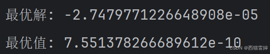
实际上对于y=x^2这样的简单函数，最小值在(0,0)点取得，这是可以提前预知的。 实际的模拟退火算法运行结果非常接近这个真实值，表明这个算法还是比较准确的。

【4】细节说明

温度只是计算的条件之一，只要没有达到最低温度。计算就从预设的解开始，不断搜索邻近的区域，在搜索的过程中，存在一定的概率会误判，但是由于温度不断变化，这种搜索会反复重复，所以基本上可以搜索全部的区域，所以大概率会获得最佳的目标值。

在条件判断中，接受概率acceptance_probability = np.exp(-delta_energy / temperature)，这一计算式的来源是：金属材料在温度T时，内部粒子自由运动能量趋于0的概率是np.exp(-delta_energy / temperature)。

【5】总结

初步学习了模拟退火算法，掌握了使用python应用模拟脱货算法获取目标函数极小值的简单方法。