目录

一、环境准备

二、数据加载与探索

三、数据预处理

四、决策树模型构建

五、模型可视化（生成决策树结构图）

六、模型预测与评估

七、超参数调优（网格搜索）

八、关键知识点解析

九、完整项目开发流程

十、常见问题解决方案

---

一、环境准备

# 安装必要库
pip install scikit-learn pandas matplotlib graphviz pydotplus

二、数据加载与探索

import pandas as pd
from sklearn.datasets import load_iris

# 加载鸢尾花数据集
iris = load_iris()
df = pd.DataFrame(iris.data, columns=iris.feature_names)
df['target'] = iris.target

# 查看数据基本信息
print(f"数据维度: {df.shape}")
print("\n前5行数据:")
print(df.head())
print("\n类别分布:")
print(df['target'].value_counts())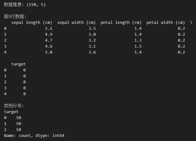

三、数据预处理

from sklearn.model_selection import train_test_split
from sklearn.preprocessing import StandardScaler

# 特征工程
X = df.iloc[:, :-1]
y = df['target']

# 划分训练集和测试集
X_train, X_test, y_train, y_test = train_test_split(X, y, test_size=0.2, random_state=42)

# 标准化处理
scaler = StandardScaler()
X_train_scaled = scaler.fit_transform(X_train)
X_test_scaled = scaler.transform(X_test)  # 注意：使用训练集的scaler

四、决策树模型构建

from sklearn.tree import DecisionTreeClassifier

# 初始化决策树分类器
dt_clf = DecisionTreeClassifier(
    criterion='gini',       # 分裂标准（基尼系数）
    max_depth=3,            # 树的最大深度
    min_samples_split=2,    # 节点分裂最小样本数
    random_state=42
)

# 模型训练
dt_clf.fit(X_train_scaled, y_train)

五、模型可视化（生成决策树结构图）

from sklearn.tree import export_graphviz
import pydotplus
from IPython.display import Image

# 导出决策树为DOT格式
dot_data = export_graphviz(
    dt_clf,
    out_file=None,
    feature_names=iris.feature_names,
    class_names=iris.target_names,
    filled=True,
    rounded=True,
    special_characters=True
)

# 生成可视化图形
graph = pydotplus.graph_from_dot_data(dot_data)
Image(graph.create_png())  # 在Jupyter中显示图片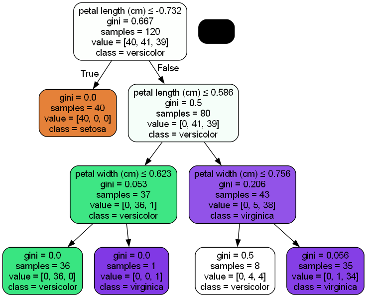

六、模型预测与评估

from sklearn.metrics import accuracy_score, confusion_matrix, classification_report

# 预测测试集
y_pred = dt_clf.predict(X_test_scaled)

# 评估指标
print(f"准确率: {accuracy_score(y_test, y_pred):.2f}")
print("\n混淆矩阵:")
print(confusion_matrix(y_test, y_pred))
print("\n分类报告:")
print(classification_report(y_test, y_pred, target_names=iris.target_names))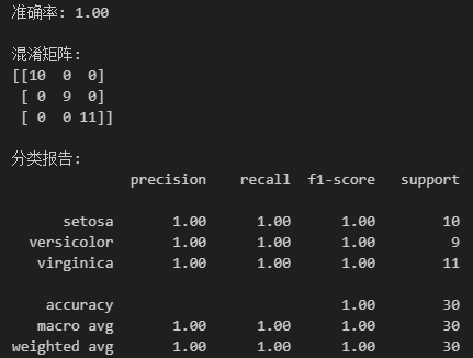

七、超参数调优（网格搜索）

from sklearn.model_selection import GridSearchCV

# 定义参数网格
param_grid = {
    'max_depth': [2, 3, 4, 5],
    'min_samples_split': [2, 5, 10],
    'criterion': ['gini', 'entropy']
}

# 网格搜索
grid_search = GridSearchCV(
    DecisionTreeClassifier(random_state=42),
    param_grid,
    cv=5,
    scoring='accuracy'
)
grid_search.fit(X_train_scaled, y_train)

# 输出最优参数
print(f"最佳参数组合: {grid_search.best_params_}")
print(f"最佳验证准确率: {grid_search.best_score_:.2f}")

# 使用最优模型预测
best_dt = grid_search.best_estimator_
y_pred_tuned = best_dt.predict(X_test_scaled)
print(f"调优后测试准确率: {accuracy_score(y_test, y_pred_tuned):.2f}")

八、关键知识点解析

特征重要性分析

import matplotlib.pyplot as plt

# 获取特征重要性
feature_importances = best_dt.feature_importances_
features = iris.feature_names

# 可视化重要性排序
plt.figure(figsize=(10,4))
plt.barh(features, feature_importances)
plt.xlabel('Feature Importance')
plt.title('决策树特征重要性分析')
plt.show()

过拟合诊断方法

• 对比训练集与测试集准确率：

train_acc = best_dt.score(X_train_scaled, y_train)
test_acc = best_dt.score(X_test_scaled, y_test)
print(f"训练集准确率: {train_acc:.2f} vs 测试集准确率: {test_acc:.2f}")

输出：

训练集准确率: 0.97 vs 测试集准确率: 1.00 

• 若训练准确率显著高于测试准确率（如0.99 vs 0.85），说明过拟合

决策边界可视化（二维示例）

import numpy as np

# 选择两个特征进行可视化
X_2d = X_train_scaled[:, [0, 2]]  # sepal length 和 petal length

# 训练简化模型
dt_2d = DecisionTreeClassifier(max_depth=3)
dt_2d.fit(X_2d, y_train)

# 生成网格点
x_min, x_max = X_2d[:, 0].min()-1, X_2d[:, 0].max()+1
y_min, y_max = X_2d[:, 1].min()-1, X_2d[:, 1].max()+1
xx, yy = np.meshgrid(np.arange(x_min, x_max, 0.02),
                     np.arange(y_min, y_max, 0.02))

# 预测并绘制
Z = dt_2d.predict(np.c_[xx.ravel(), yy.ravel()])
Z = Z.reshape(xx.shape)

plt.contourf(xx, yy, Z, alpha=0.4)
plt.scatter(X_2d[:,0], X_2d[:,1], c=y_train, s=20, edgecolor='k')
plt.xlabel('标准化后的花萼长度')
plt.ylabel('标准化后的花瓣长度')
plt.title('决策树分类边界可视化')
plt.show()

九、完整项目开发流程

1. 业务场景适配

   • 金融风控：客户信用评估

   • 医疗诊断：疾病分类预测

   • 工业制造：产品质量检测

2. 生产级代码优化

# 模型持久化
import joblib

# 保存标准化器和模型
joblib.dump(scaler, 'std_scaler.pkl')
joblib.dump(best_dt, 'dt_model.pkl')

# 新数据预测示例
new_data = [[5.1, 3.5, 1.4, 0.2]]  # 原始数据
loaded_scaler = joblib.load('std_scaler.pkl')
loaded_model = joblib.load('dt_model.pkl')

scaled_data = loaded_scaler.transform(new_data)
prediction = loaded_model.predict(scaled_data)
print(f"预测类别: {iris.target_names[prediction[0]]}")

十、常见问题解决方案

处理类别不平衡问题

# 设置类别权重
balanced_dt = DecisionTreeClassifier(
    class_weight='balanced',  # 自动调整权重
    max_depth=4,
    random_state=42
)

处理缺失值

from sklearn.impute import SimpleImputer

# 在预处理阶段添加缺失值处理
imputer = SimpleImputer(strategy='median')
X_train_imputed = imputer.fit_transform(X_train)
X_test_imputed = imputer.transform(X_test)

处理高维数据

# 结合PCA降维
from sklearn.decomposition import PCA

pca = PCA(n_components=0.95)  # 保留95%方差
X_train_pca = pca.fit_transform(X_train_scaled)
X_test_pca = pca.transform(X_test_scaled)

---

实战建议：

1. 尝试更换其他数据集（如泰坦尼克生存预测、糖尿病预测）

2. 对比不同树模型（随机森林 vs 决策树）

3. 部署为Flask/Django API服务

4. 使用SHAP库进行模型解释：

pip install shap

import shap

explainer = shap.TreeExplainer(best_dt)
shap_values = explainer.shap_values(X_test_scaled)
shap.summary_plot(shap_values, X_test_scaled, feature_names=iris.feature_names)