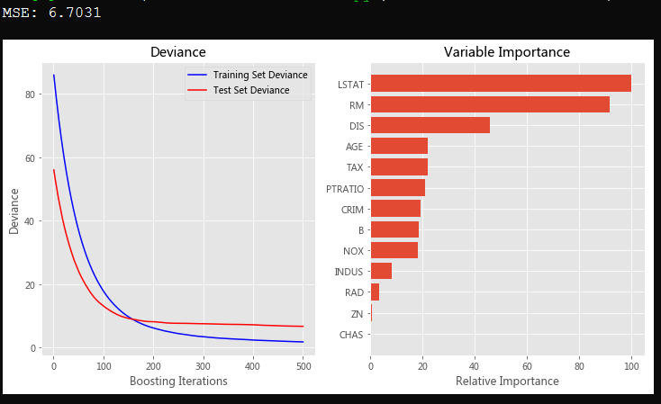
# -*- coding: utf-8 -*-
"""
Created on Wed May  9 09:53:30 2018

@author: admin
"""

import numpy as np
import matplotlib.pyplot as plt

from sklearn import ensemble
from sklearn import datasets
from sklearn.utils import shuffle
from sklearn.metrics import mean_squared_error

# #############################################################################
# Load data
boston = datasets.load_boston()
X, y = shuffle(boston.data, boston.target, random_state=13)
X = X.astype(np.float32)
offset = int(X.shape[0] * 0.9)
X_train, y_train = X[:offset], y[:offset]
X_test, y_test = X[offset:], y[offset:]

# #############################################################################
# Fit regression model
params = {'n_estimators': 500, 'max_depth': 4, 'min_samples_split': 2,
          'learning_rate': 0.01, 'loss': 'ls'}   #随便指定参数长度,也不用在传参的时候去特意定义一个数组传参
clf = ensemble.GradientBoostingRegressor(**params)

clf.fit(X_train, y_train)
mse = mean_squared_error(y_test, clf.predict(X_test))
print("MSE: %.4f" % mse)

# #############################################################################
# Plot training deviance

# compute test set deviance
test_score = np.zeros((params['n_estimators'],), dtype=np.float64)

for i, y_pred in enumerate(clf.staged_predict(X_test)):
    test_score[i] = clf.loss_(y_test, y_pred)

plt.figure(figsize=(12, 6))
plt.subplot(1, 2, 1)
plt.title('Deviance')
plt.plot(np.arange(params['n_estimators']) + 1, clf.train_score_, 'b-',
         label='Training Set Deviance')
plt.plot(np.arange(params['n_estimators']) + 1, test_score, 'r-',
         label='Test Set Deviance')
plt.legend(loc='upper right')
plt.xlabel('Boosting Iterations')
plt.ylabel('Deviance')

# #############################################################################
# Plot feature importance
feature_importance = clf.feature_importances_
# make importances relative to max importance
feature_importance = 100.0 * (feature_importance / feature_importance.max())
sorted_idx = np.argsort(feature_importance)
pos = np.arange(sorted_idx.shape[0]) + .5
plt.subplot(1, 2, 2)
plt.barh(pos, feature_importance[sorted_idx], align='center')
plt.yticks(pos, boston.feature_names[sorted_idx])
plt.xlabel('Relative Importance')
plt.title('Variable Importance')
plt.show()
房产数据介绍:
- CRIM per capita crime rate by town
- ZN proportion of residential land zoned for lots over 25,000 sq.ft.
- INDUS proportion of non-retail business acres per town
- CHAS Charles River dummy variable (= 1 if tract bounds river; 0 otherwise)
- NOX nitric oxides concentration (parts per 10 million)
- RM average number of rooms per dwelling
- AGE proportion of owner-occupied units built prior to 1940
- DIS weighted distances to five Boston employment centres
- RAD index of accessibility to radial highways
- TAX full-value property-tax rate per $10,000
- PTRATIO pupil-teacher ratio by town
- B 1000(Bk - 0.63)^2 where Bk is the proportion of blacks by town
- LSTAT % lower status of the population
- MEDV Median value of owner-occupied homes in $1000's
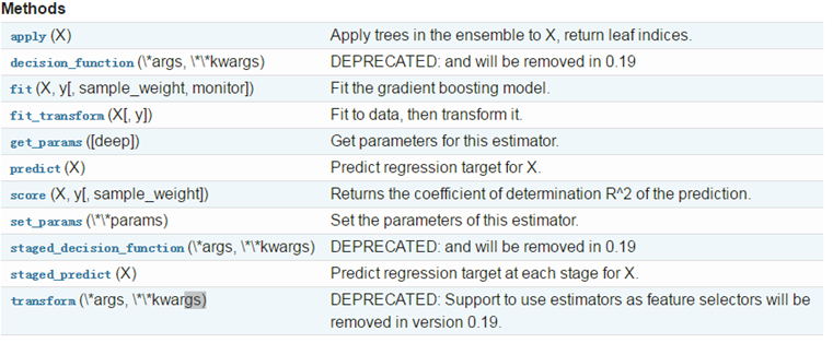
方法: