图像退化/复原过程的模型
退化:由于成像系统各种 因素的影响,使得图像质量降低
噪声模型
- 一些重要的噪声
高斯噪声
瑞利噪声
伽马(爱尔兰)噪声
指数分布噪声
均匀分布噪声
脉冲噪声(椒盐噪声)
- 几种噪声的运用
高斯噪声源于电子电路噪声和由低照明度或 高温带来的传感器噪声
瑞利噪声对分布在图像范围内特征化噪声有 用
伽马分布和指数分布用于激光成像噪声
均匀密度分布作为模拟随机数产生器的基础
脉冲噪声用于成像中的短暂停留中,如错误 的开关操作
空间域滤波复原(唯一退化是噪声)
图像复原的空间滤波器(滤噪声)
CDF:累积分布函数
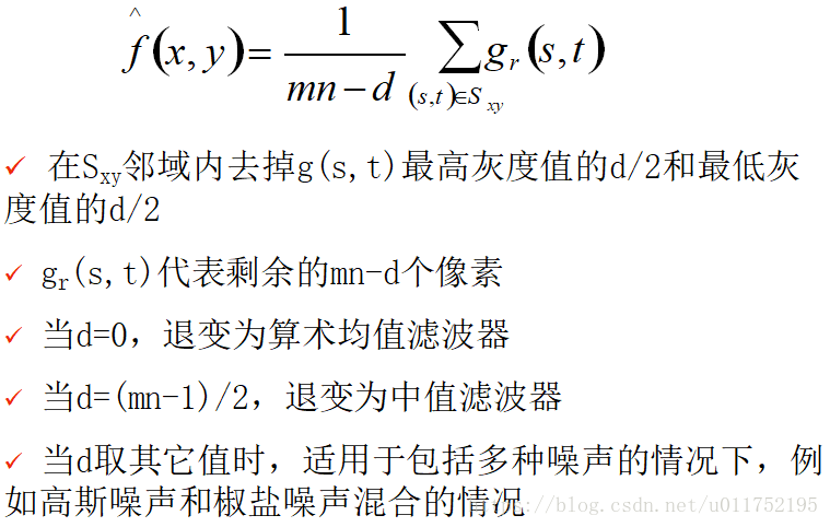
1、均值滤波器:
处理高斯或均匀等随机噪声:算术均值滤波器、几何均值滤波器(与算术均值滤波器相比,会丢失更少的图像细节——相对锐化)、谐波均值滤波 器(“盐”噪声效果好、善于处理高斯噪声)、逆谐波均值滤波器(Q为正数时,消除“胡椒”噪声;Q为负数时,消除“盐”噪声)
2、顺序统计滤波器:
中值滤波器(相同尺寸下,比均值滤波器引起的模糊少;对单极或双极脉冲噪声非常有效)、

最大值滤波器(用于发现最亮点;有效过滤“胡椒”噪声(“胡椒”噪声 是非常低的值))、
最小值滤波器(用于发现最暗点;有效过滤“盐”噪声(“盐”噪声 是非常低的值))、
中点 滤波器高斯和均匀随机分布这类噪声有最好的 效果)、
修正后的阿尔法均值滤波器:
自适应滤波器:自适应局部噪声消除滤波器、自适应中值滤波器;到PPT341
噪声产生:
>> g=imnoise(f,'gaussian',0,1); 高斯噪声
>> r=imnoise2('gaussian',100000,1,0,1); %自定义
>> hist(r,50) %直方图
估计噪声参数
频域:傅里叶谱周期; 空间域:平均值、方差;MATLAB代码:statmoments(计算平均值和中心距)
%估计噪声参数
f=imread('44.tif');
[b,c,r]=roipoly(f);
subplot(2,2,1),imshow(f) %显示模板
subplot(2,2,2),imshow(b) %显示模板
[h,npix]=histroi(f,c,r);
subplot(2,2,3),bar(h,1) %roi直方图
[v,unv]=statmoments(h,2); %b区域均值方差
x=imnoise2('gaussian',npix,1,147,20);
subplot(2,2,4),hist(x,130)%高斯直方图
MATLAB
- 空间噪声滤波器
%空间滤波-spfilt
f=imread('219.tif');
subplot(3,2,1),imshow(f)
[m,n]=size(f);
r=imnoise2('salt & pepper',m,n,0.1,0);
subplot(3,2,2),imshow(r)
gp=f;
gp(r==0)=0; %叠加胡椒
subplot(3,2,3),imshow(gp)
r=imnoise2('salt & pepper',m,n,0,0.1);
gs=f;
gs(r==1)=255; %叠加盐
subplot(3,2,4),imshow(gs)
fp=spfilt(gp,'chmean',3,3,1.5); %Q+反调和滤波器-适合胡椒
subplot(3,2,5),imshow(fp)
fs=spfilt(gs,'chmean',3,3,-1.5); %Q-反调和滤波器-适合盐
subplot(3,2,6),imshow(fs) 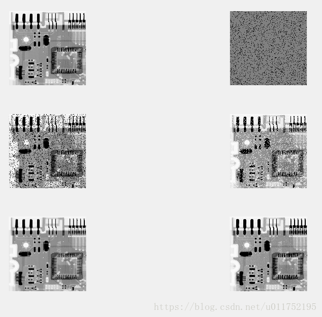
- 自适应
%自适应滤波
f=imread('219.tif');
subplot(2,2,1),imshow(f)
g=imnoise(f,'salt & pepper',.25);
subplot(2,2,2),imshow(g)
f1=medfilt2(g,[7 7],'symmetric');
subplot(2,2,3),imshow(f1)
f2=adpmedian(g,7);
subplot(2,2,4),imshow(f2) 
- 退化(模拟设备的图像退化)
%退化函数建模
f=checkerboard(8);
subplot(2,2,1);imshow(f);title("8X8棋盘");
psf=fspecial('motion',7,45);
subplot(2,2,2);imshow(psf);title("运动模糊滤波器");
gb=imfilter(f,psf,'circular');
subplot(2,2,3);imshow(gb);title("退化图像");
noise=imnoise2('Gaussian',size(f,1),size(f,2),0,sqrt(0.001));%高斯噪声
g=gb+noise;
subplot(2,2,4);imshow(g);title("退化+噪声");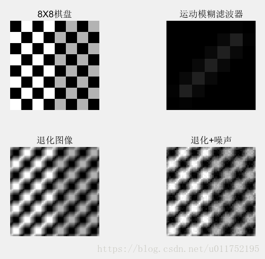
频率域滤波复原(削减周期噪声)
带阻滤波器:理想带阻滤波器、巴特沃思带阻滤波器、高斯带阻滤波器
带通滤波器
陷波滤波器
最佳陷波滤波器
线性图像复原
- 约束的最小二乘法
- 维纳滤波(最小均方差 逆滤波 复原退化 )
%维纳滤波 续例4.7 deconvwnr函数
subplot(2,2,1),imshow(g),title("退化图像");
frest1=deconvwnr(g,psf);
subplot(2,2,2),imshow(frest1),title("直接逆滤波");
Sn=abs(fft2(noise)).^2;
nA=sum(Sn(:))/numel(noise);
Sf=abs(fft2(f)).^2;
fA=sum(Sf(:))/numel(f);
R=nA/fA;
frest2=deconvwnr(g,psf,R);
subplot(2,2,3),imshow(frest2),title("常数维纳滤波");
ncorr=fftshift(real(ifft2(Sn)));
icorr=fftshift(real(ifft2(Sf)));
frest3=deconvwnr(g,psf,ncorr,icorr);
subplot(2,2,4),imshow(frest3),title("自相关维纳滤波");
非线性图像复原
- 露西-查理德森算法的迭代非线性复原
%露西-查理德森算法 非线性复原 deconvlucy函数
g=checkerboard(8);
subplot(2,2,1),imshow(pixeldup(g,8)),title("退化图像");;
psf=fspecial('gaussian',7,10);
sd=0.01;
g=imnoise(imfilter(g,psf),'gaussian',0,sd^2);
subplot(2,2,2),imshow(g),title("退化噪声图像");
dampar=10*sd;
lim=ceil(size(psf,1)/2);
weight=zeros(size(g));
weight(lim+1:end-lim,lim+1:end-lim)=1;
numit=5; %迭代次数
f5=deconvlucy(g,psf,numit,dampar,weight);
subplot(2,2,3),imshow(pixeldup(f5,8),[]),title("露西迭代=5");
f20=deconvlucy(g,psf,20,dampar,weight);
subplot(2,2,4),imshow(pixeldup(f20,8),[]),title("露西迭代=20");

来自投影的图像重建(CT图像配准)
radon-由二维图像产生投影
%投影重建 函数radon
g1=zeros(600,600);
g1(100:500,250:350)=1;
g2=phantom('Modified Shepp-Logan',600);
subplot(2,2,1),imshow(g1)
subplot(2,2,2),imshow(g2)
theta=0:0.5:179.5;
[R1,xp1]=radon(g1,theta);
[R2,xp2]=radon(g2,theta);
R1=flipud(R1');
R2=flipud(R2');
subplot(2,2,3),imshow(R1,[],'XData',xp1([1 end]),'YData',[179.5 0])
axis xy
axis on
xlabel('\rho'),ylabel('\theta')
subplot(2,2,4),imshow(R2,[],'XData',xp2([1 end]),'YData',[179.5 0])
axis xy
axis on
xlabel('\rho'),ylabel('\theta')
iradon-由投影 产生二维图像