0:环境
本教程的环境是Python2.7、Keras+Tensorflow、sklearn、matplotlib、numpy
Ubuntu18.
1:原理
LeNet结构是LeCun在1998年提出了神经网络结构。本结构在OCR文字识别方面有较大优势,识别精度较高。
网络的结构是:INPUT => CONV => ACT => POOL => CONV => ACT => POOL => FC => ACT => FC => SOFTMAX
见下表:
| Layer Type | Output Size | Filter Size / Stride |
| INPUT IMAGE | 28 x 28 x 1 | |
| CONV | 28 x 28 x 20 | 5 x 5, K = 20 |
| ACT | 28 x 28 x 20 | |
| POOL | 14 x 14 x 20 | 2 x 2 |
| CONV | 14 x 14 x 50 | 5 x 5, K = 50 |
| ACT | 14 x 14 x 50 | |
| POOL | 7 x 7 x 50 | 2 x 2 |
| FC | 500 | |
| ACT | 500 | |
| FC | 10 | |
| SOFTMAX | 10 |
输入层是28 x 28 x 1的黑白图片。
第二层是 28 x 28 x 20的大小,生成方式是使用20个5 x 5的filter分别对输入图片进行卷积。与神经网络类似,每个点都有自身的激活函数。同时带有POOLING(池化层),本层的Filter矩阵是2 x 2。每2 x 2之间只留下一个最大值自上到下从左到右的处理,POOL的输出尺寸只有输入的1/4大小。
第三层也是CONV + ACT + POOL的形式。
第四层是全连接的500个神经元。全连接的意思是,第三层的全部输入都分别和第四层的每个神经元相连。假如不说明FC,则默认两层之间的连接线,有一定概率会失去连接。
第五层是输出层。
2:代码
有两个文件,分别是lenet.py和lenet_mnist.py。放在同一个目录即可。
2.1 lenet.py
# import the necessary packages
from keras.models import Sequential
from keras.layers.convolutional import Conv2D
from keras.layers.convolutional import MaxPooling2D
from keras.layers.core import Activation
from keras.layers.core import Flatten
from keras.layers.core import Dense
from keras import backend as K

class LeNet:
	@staticmethod
	def build(width, height, depth, classes):
		# initialize the model
		model = Sequential()
		inputShape = (height, width, depth)

		# if we are using "channels first", update the input shape
		if K.image_data_format() == "channels_first":
			inputShape = (depth, height, width)

		# first set of CONV => RELU => POOL layers
		model.add(Conv2D(20, (5, 5), padding="same",
			input_shape=inputShape))
		model.add(Activation("relu"))
		model.add(MaxPooling2D(pool_size=(2, 2), strides=(2, 2)))

		# second set of CONV => RELU => POOL layers
		model.add(Conv2D(50, (5, 5), padding="same"))
		model.add(Activation("relu"))
		model.add(MaxPooling2D(pool_size=(2, 2), strides=(2, 2)))

		# first (and only) set of FC => RELU layers
		model.add(Flatten())
		model.add(Dense(500))
		model.add(Activation("relu"))

		# softmax classifier
		model.add(Dense(classes))
		model.add(Activation("softmax"))

		# return the constructed network architecture
		return model
2.2 lenet_mnist.py
# import the necessary packages
from lenet import LeNet
from keras.optimizers import SGD
from sklearn.preprocessing import LabelBinarizer
from sklearn.model_selection import train_test_split
from sklearn.metrics import classification_report
from sklearn import datasets
from keras import backend as K
import matplotlib.pyplot as plt
import numpy as np
import os
# grab the MNIST dataset (if this is your first time using this
# dataset then the 55MB download may take a minute)
print("[INFO] accessing MNIST...")
#dataset = datasets.fetch_mldata("MNIST Original")
path1 = os.path.dirname(os.path.abspath(__file__))
dataset = datasets.fetch_mldata("MNIST Original", data_home=path1)
data = dataset.data
# if we are using "channels first" ordering, then reshape the
# design matrix such that the matrix is:
# num_samples x depth x rows x columns
if K.image_data_format() == "channels_first":
data = data.reshape(data.shape[0], 1, 28, 28)
# otherwise, we are using "channels last" ordering, so the design
# matrix shape should be: num_samples x rows x columns x depth
else:
data = data.reshape(data.shape[0], 28, 28, 1)
# scale the input data to the range [0, 1] and perform a train/test
# split
(trainX, testX, trainY, testY) = train_test_split(data / 255.0,
dataset.target.astype("int"), test_size=0.25, random_state=42)
# convert the labels from integers to vectors
le = LabelBinarizer()
trainY = le.fit_transform(trainY)
testY = le.transform(testY)
# initialize the optimizer and model
print("[INFO] compiling model...")
opt = SGD(lr=0.01)
model = LeNet.build(width=28, height=28, depth=1, classes=10)
model.compile(loss="categorical_crossentropy", optimizer=opt,
metrics=["accuracy"])
# train the network
print("[INFO] training network...")
H = model.fit(trainX, trainY, validation_data=(testX, testY),
batch_size=128, epochs=20, verbose=1)
# evaluate the network
print("[INFO] evaluating network...")
predictions = model.predict(testX, batch_size=128)
print(classification_report(testY.argmax(axis=1),
predictions.argmax(axis=1),
target_names=[str(x) for x in le.classes_]))
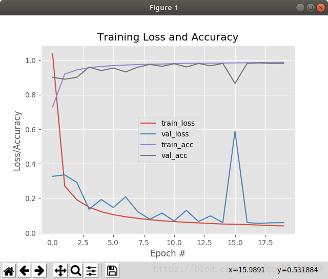
# plot the training loss and accuracy
plt.style.use("ggplot")
plt.figure()
plt.plot(np.arange(0, 20), H.history["loss"], label="train_loss")
plt.plot(np.arange(0, 20), H.history["val_loss"], label="val_loss")
plt.plot(np.arange(0, 20), H.history["acc"], label="train_acc")
plt.plot(np.arange(0, 20), H.history["val_acc"], label="val_acc")
plt.title("Training Loss and Accuracy")
plt.xlabel("Epoch #")
plt.ylabel("Loss/Accuracy")
plt.legend()
plt.show()初次运行以下代码,初次调用sklearn的fetch_mldata会在本文件的目录内生成mldata文件夹,并把MNIST的dataset下载到该目录内。只有50多MB,但是速度和机器性能、网络有关。
path1 = os.path.dirname(os.path.abspath(__file__))
dataset = datasets.fetch_mldata("MNIST Original", data_home=path1)
3:运行结果
[INFO] evaluating network...
             precision    recall  f1-score   support

          0       0.99      0.99      0.99      1677
          1       0.99      0.99      0.99      1935
          2       0.98      0.99      0.98      1767
          3       0.99      0.97      0.98      1766
          4       0.98      0.99      0.99      1691
          5       0.99      0.97      0.98      1653
          6       0.99      0.99      0.99      1754
          7       0.99      0.98      0.98      1846
          8       0.94      0.98      0.96      1702
          9       0.98      0.97      0.98      1709

avg / total       0.98      0.98      0.98     17500
可以达到98%的精度,数据十分可观。
我的电脑是i3-6100的CPU,需要90秒才能完成一次迭代,没有GPU。书本的作者的CPU要30秒,GPU只要3秒。
所以,TODO:在GPU上跑
参考资料(也是代码来源):Deep.Learning.for.Computer.Vision.with.Python.Starter.Bundle.pdf